Dask example
This material is adapted from the Dask tutorial documentation and the Earth and Environmental Data Science website.
Note
A Dask array looks and feels a lot like a Numpy array.
However, a dask array doesn’t directly hold any data. Instead, it symbolically represents the computations needed to generate the data.
Nothing is actually computed until the actual numerical values are needed. This mode of operation is called “lazy”; it allows one to build up complex, large calculations symbolically before turning them over the scheduler for execution.
If we want to create a Numpy array of all ones, we do it like this:
import numpy as np
shape = (1000, 4000)
ones_np = np.ones(shape)
ones_np
array([[1., 1., 1., ..., 1., 1., 1.],
       [1., 1., 1., ..., 1., 1., 1.],
       [1., 1., 1., ..., 1., 1., 1.],
       ...,
       [1., 1., 1., ..., 1., 1., 1.],
       [1., 1., 1., ..., 1., 1., 1.],
       [1., 1., 1., ..., 1., 1., 1.]])
This array contains exactly 32 MB of data:
ones_np.nbytes / 1e6
32.0
Now let’s create the same array using dask’s array interface.
import dask.array as da

ones = da.ones(shape)
ones
|
The dask array representation reveals the concept of “chunks”.
Note
“Chunks” describes how the array is split into sub-arrays. We did not specify any chunks, so Dask just used one single chunk for the array. This is not much different from a Numpy array at this point.
Specifying Chunks
However, we could have split up the array into many chunks.
 source: Dask Array Documentation
There are several ways to specify chunks.
Here, we will use a block shape.
chunk_shape = (1000, 1000)
ones = da.ones(shape, chunks=chunk_shape)
ones
|
Notice that we just see a symbolic representation of the array, including its:
shape,
dtype, and
chunksize.
No data has been generated yet.
When we call .compute() on a Dask array, the computation is trigger and the Dask array becomes a Numpy array.
ones.compute()
array([[1., 1., 1., ..., 1., 1., 1.],
       [1., 1., 1., ..., 1., 1., 1.],
       [1., 1., 1., ..., 1., 1., 1.],
       ...,
       [1., 1., 1., ..., 1., 1., 1.],
       [1., 1., 1., ..., 1., 1., 1.],
       [1., 1., 1., ..., 1., 1., 1.]])
In order to understand what happened when we called .compute(), we can visualize the Dask graph, the symbolic operations that make up the array
ones.visualize()
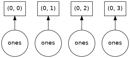
Our array has four chunks. To generate it, dask calls np.ones four times and then concatenates this together into one array.
Rather than immediately loading a dask array (which puts all the data into RAM), it is more common to want to reduce the data somehow. For example
sum_of_ones = ones.sum()
sum_of_ones.visualize()
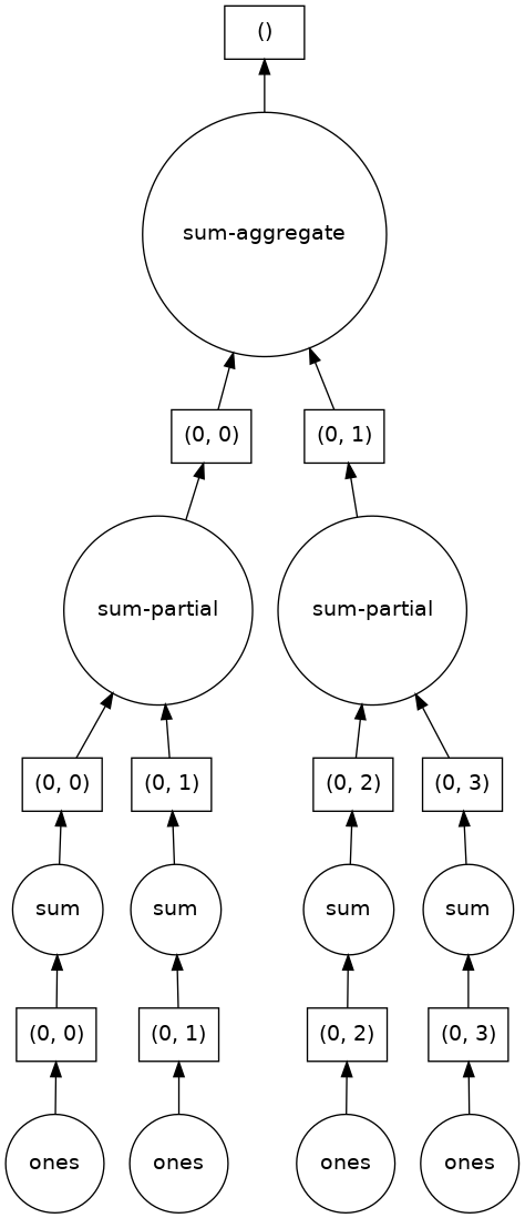
Here we see Dask’s strategy for finding the sum.
This simple example illustrates the beauty of Dask: it automatically designs an algorithm appropriate for custom operations with big data.
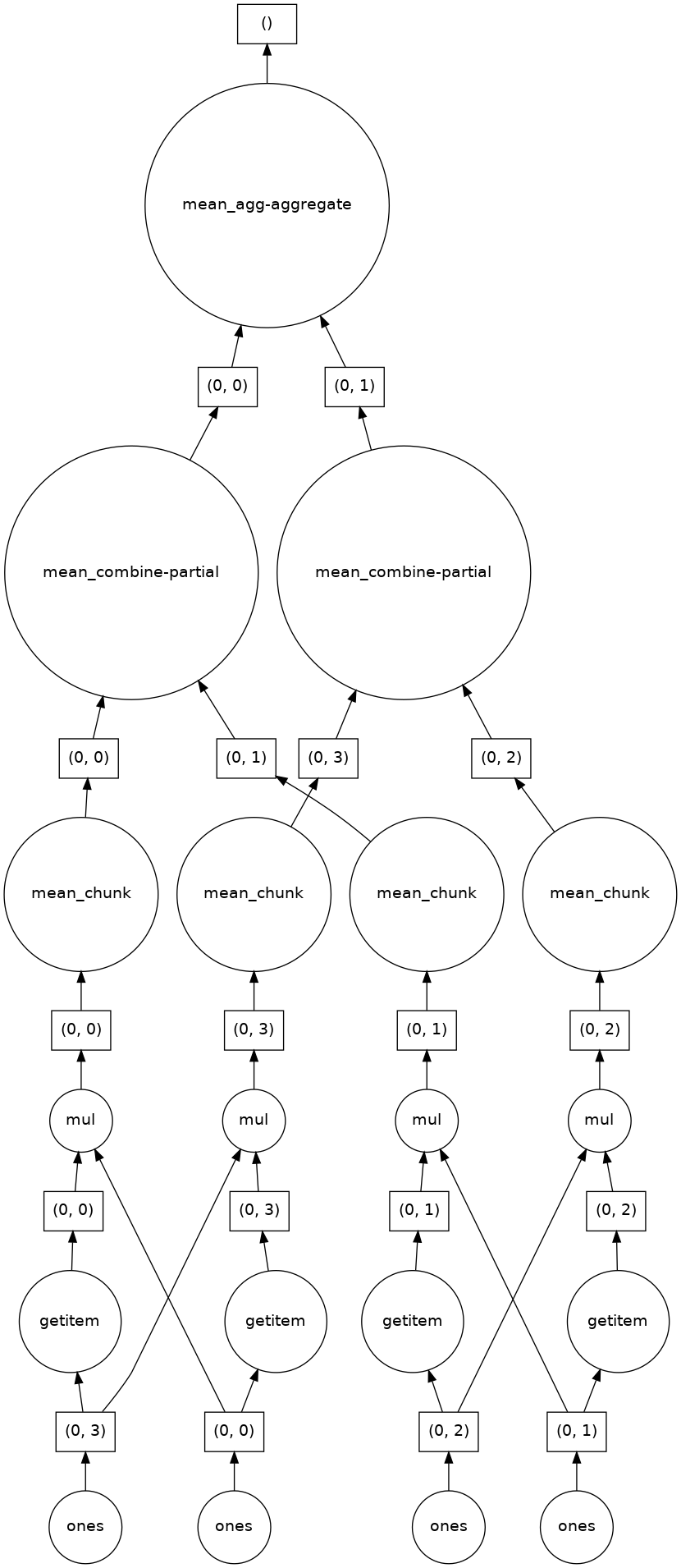
If we make our operation more complex, the graph gets more complex.
fancy_calculation = (ones * ones[::-1, ::-1]).mean()
fancy_calculation.visualize()
A Bigger Calculation
The examples above were toy examples; the data (32 MB) is nowhere nearly big enough to warrant the use of dask.
We can make it a lot bigger!
bigshape = (200000, 4000)

big_ones = da.ones(bigshape, chunks=chunk_shape)
big_ones
|
big_ones.nbytes / 1e6
6400.0
This dataset is 6.4 GB, rather MB! This is probably close to or greater than the amount of available RAM than you have in your computer. Nevertheless, Dask has no problem working on it.
Danger
Do not try to .visualize() this array!
When doing a big calculation, Dask also has some tools to help us understand what is happening under the hood
from dask.diagnostics import ProgressBar

big_calc = (big_ones * big_ones[::-1, ::-1]).mean()

with ProgressBar():
    result = big_calc.compute()
result
[ ] | 0% Completed | 0.0s
[# ] | 3% Completed | 0.1s
[### ] | 9% Completed | 0.2s
[##### ] | 12% Completed | 0.3s
[###### ] | 17% Completed | 0.4s
[######## ] | 21% Completed | 0.5s
[########## ] | 27% Completed | 0.6s
[############# ] | 32% Completed | 0.7s
[############### ] | 38% Completed | 0.8s
[################# ] | 44% Completed | 0.9s
[################### ] | 49% Completed | 1.0s
[###################### ] | 55% Completed | 1.1s
[######################## ] | 61% Completed | 1.2s
[########################## ] | 67% Completed | 1.3s
[############################# ] | 73% Completed | 1.4s
[############################### ] | 79% Completed | 1.5s
[################################# ] | 84% Completed | 1.6s
[#################################### ] | 90% Completed | 1.7s
[###################################### ] | 95% Completed | 1.8s
[########################################] | 100% Completed | 1.9s
1.0
Reduction
All the usual Numpy methods work on Dask arrays.
You can also apply numpy function directly to a Dask array, and it will stay lazy.
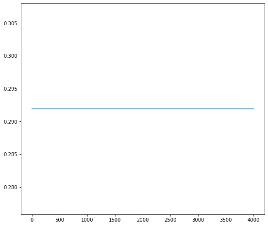
big_ones_reduce = (np.cos(big_ones)**2).mean(axis=0)
big_ones_reduce
|
Plotting also triggers computation, since we need the actual values
from matplotlib import pyplot as plt
%matplotlib inline
plt.rcParams['figure.figsize'] = (9,8)
plt.plot(big_ones_reduce)
[<matplotlib.lines.Line2D at 0x7fc6381faf40>]
Distributed Cluster
For more fancy visualization of what Dask is doing, we can use the distributed scheduler.
from dask.distributed import Client, LocalCluster
cluster = LocalCluster()
client = Client(cluster)
client
Client
|
Cluster
|
big_calc.compute()
1.0
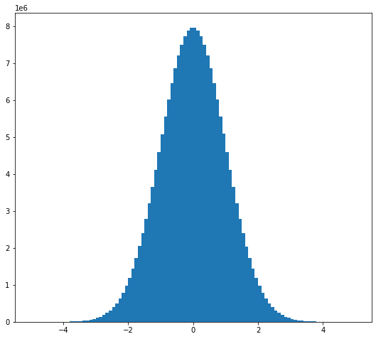
random_values = da.random.normal(size=(2e8,), chunks=(1e6,))
hist, bins = da.histogram(random_values, bins=100, range=[-5, 5])
hist
|
x = 0.5 * (bins[1:] + bins[:-1])
width = np.diff(bins)
hist_c = hist.compute()
plt.bar(x, hist_c, width);
Dask + XArray
Important
Everything has been commented below to speed-up the Jupyter-book creation!
Xarray can automatically wrap its data in Dask arrays.
This capability turns Xarray into an extremely powerful tool for Big Data Environmental science!!!
To see this in action, we will download a fairly large dataset to analyze.
This file contains 1 year of daily data from the AVISO sea-surface height satellite altimetry dataset.
#! wget http://www.ldeo.columbia.edu/~rpa/aviso_madt_2015.tar.gz
#! tar -xvzf aviso_madt_2015.tar.gz
#! ls 2015 | wc -l
Let’s load the first file as a regular xarray dataset.
#import xarray as xr
# ds_first = xr.open_dataset('2015/dt_global_allsat_madt_h_20150101_20150914.nc')
# ds_first
# ds_first.nbytes / 1e6
This one file is about 8 MB. So 365 of them will be nearly 3 GB. If we had downloaded all 25 years of data, it would be 73 GB. This is a good example of “medium data.”
open_mfdataset
We already saw an incredibly useful function in xarray is open_mfdataset.
Using open_mfdataset we can easily open all the netcdf files into one Dataset object.
Tip
If you got a “Too many open files” OSError. You will have to increase your ulimit from the command line before launching the notebook:
$ ulimit -S -n 4000
# ds = xr.open_mfdataset('2015/*.nc')
# ds
Note that the values are not displayed, since that would trigger computation.
# ssh = ds.adt
# ssh
# ssh[0].plot()
# ssh_2015_mean = ssh.mean(dim='time')
# ssh_2015_mean.load()
# ssh_2015_mean.plot()
# ssh_anom = ssh - ssh_2015_mean
# ssh_variance_lonmean = (ssh_anom**2).mean(dim=('lon', 'time'))
# ssh_variance_lonmean.plot()
# weight = np.cos(np.deg2rad(ds.lat))
# weight /= weight.mean()
# (ssh_anom * weight).mean(dim=('lon', 'lat')).plot()
Cloud Storage
Since we are in the cloud, we can also skip the whole “download” step and just work with data stored directly in cloud storage.
There are a lot of different pieces that make this work:
We don’t have time to go over them all.
But here is an example from Pangeo:
from intake import open_catalog

cat = open_catalog("https://raw.githubusercontent.com/pangeo-data/pangeo-datastore/master/intake-catalogs/ocean.yaml")
list(cat)
['sea_surface_height',
 'cesm_mom6_example',
 'ECCOv4r3',
 'SOSE',
 'GODAS',
 'ECCO_layers',
 'altimetry',
 'LLC4320',
 'GFDL_CM2_6',
 'CESM_POP',
 'channel',
 'MEOM_NEMO']
# ds = cat["sea_surface_height"].to_dask()
# ds
# ds.sla.data