Comparisons between Reefs¶

Notebook designed by Mark Hammerton from AIMS

import os
import numpy as np
import pandas as pd
from scipy import stats
from scipy.spatial import cKDTree

import urllib.request
import datetime as dt

import netCDF4
from netCDF4 import Dataset, num2date

from matplotlib import pyplot as plt
# %config InlineBackend.figure_format = 'retina'
plt.ion()  # To trigger the interactive inline mode

In this notebook, we use the AIMS eReefs extraction tool to extract time series data for two locations of interest.

Example problem: How strong does the wind need to be to set the direction of the surface ocean currents?¶

We will investigate the relationship between the strength of the wind and the direction of the surface currents for two locations. We will look at Myrmidon Reef, which is on the far outer edge of the GBR and is almost right in the middle of the southern Eastern Australian Current.

Our second location will be Davies Reef which is further in the reef matrix, but in a similar sector of the GBR.

Analysis method¶

The East Australian Current (EAC) usually is a strong southward current near Myrmidon and Davies Reefs. During winter months the wind moves in a north eastern direction in the near opposite direction to the EAC. When the wind is low the surface currents are dominated by the EAC. As the wind picks up at some speed the wind overpowers the EAC and the surface current moves in the direction of the wind.

To determine the relation between the wind and the surface currents we will pull out hourly time series wind and current data for our two locations of interest. We will then look at the correlation between the wind and current vectors, where a correlation of 1 indicates they are pointing in the same direction, and -1 indicated they are in opposite directions.

Setting up to get the data¶

To extract the time series data using the extraction tool we need to create a CSV file containing the sites of interest. This file needs to contain the coordinates and names of the sites. To create this I first added my points manually in Google Earth. This was done to simply get the location of Myrmidon and Davies Reefs. Using Google Earth to create your CSV file for the extraction tool is only useful if you don’t already know the coordinates of your sites.

The location of the two sites are:

name,lat,lon
Myrmidon Reef,-18.265599,147.389028
Davies Reef,-18.822840,147.645209

Extracting the data¶

The CSV file] was uploaded to the AIMS extraction tool and the extraction was performed with the following settings:

Data collection: GBR1 Hydro (Version 2) Variables: Eastward wind speed (wspeed_u), Northward wind speed (wspeed_v), Northward current (v), Eastward current (u) Date range: 1 January 2019 - 31 December 2019 Time step: hourly Depths: -2.35 m

Once the extraction request was submitted the dataset was created after an one hour of processing the data was available for download from Extraction request: Example dataset: Wind-vs-Current at Davies and Myrmidon Reefs (2019).

Downloading the data¶

In this notebook we will download the data using scripting. There is no need to re-run the extraction request as each extraction performed by the extraction tool has a permanent public page created for it that can be used to facilitate sharing of the data.

Let’s first create a temporary folder to contain the downloaded data. Note: The temp folder is excluded using the .gitignore so it is not saved to the code repository, which is why we must reproduce it.

if not os.path.exists('temp'):
    os.makedirs('temp')

Now let’s download the data. The file to download is 12.9 MB and so this download might take a little while. To allow us to re-run this script without having to wait for the download each time we first check that the download has not already been done.

extractionfile = os.path.join('temp','2009.c451dc3-collected.csv')  # Use os.path.join so the script will work cross-platform

if not os.path.exists(extractionfile):
    print("Downloading extraction data ...")
    url = 'https://api.ereefs.aims.gov.au/data-extraction/request/2009.c451dc3/files/2009.c451dc3-collected.csv'
    req = urllib.request.urlretrieve(url, extractionfile)
    print(req)
else:
    print("Skipping redownloading extraction data")

Downloading extraction data ...

('temp/2009.c451dc3-collected.csv', <http.client.HTTPMessage object at 0x7f5bd3d10430>)

Reading and cleaning the data¶

Read the resulting CSV file into a Pandas data frame.

df = pd.read_csv(extractionfile)
df.head()

	Aggregated Date/Time	Variable	Depth	Site Name	Latitude	Longitude	mean	median	p5	p95	lowest	highest
0	2019-01-01T00:00	wspeed_u	99999.90	Myrmidon Reef	-18.265599	147.389028	-9.568488	-9.568488	-9.568488	-9.568488	-9.568488	-9.568488
1	2019-01-01T00:00	wspeed_u	99999.90	Davies Reef	-18.822840	147.645209	-8.880175	-8.880175	-8.880175	-8.880175	-8.880175	-8.880175
2	2019-01-01T00:00	wspeed_v	99999.90	Myrmidon Reef	-18.265599	147.389028	3.260430	3.260430	3.260430	3.260430	3.260430	3.260430
3	2019-01-01T00:00	wspeed_v	99999.90	Davies Reef	-18.822840	147.645209	2.756750	2.756750	2.756750	2.756750	2.756750	2.756750
4	2019-01-01T00:00	v	-2.35	Myrmidon Reef	-18.265599	147.389028	0.047311	0.047311	0.047311	0.047311	0.047311	0.047311

Here we can see that data is in tidy format. That is each observation is in one row per time step, variable, depth and site. For each of these combinations there are summary statistics corresponding to the aggregation process that was applied. Somewhat confusingly we extracted hourly data from the hourly eReefs hydrodynamic model and so there was no aggregation applied. As a result all the stats values are the same and the mean corresponds to the actual extracted data values. Let’s clean this up a little by removing the redundant columns. Here we also drop the depth variable as the depth of the wind doesn’t match the depth of the surface current and so makes it difficult to align the wind and the current together. Since we are only processing a single depth this is an OK simplification. If we were processing the current at multiple depths then we would need a more complex set of data wraggling.

df2 = df.drop(columns=['median', 'p5', 'p95', 'lowest','highest','Depth']).rename(columns={"mean": "value"})
df2

	Aggregated Date/Time	Variable	Site Name	Latitude	Longitude	value
0	2019-01-01T00:00	wspeed_u	Myrmidon Reef	-18.265599	147.389028	-9.568488
1	2019-01-01T00:00	wspeed_u	Davies Reef	-18.822840	147.645209	-8.880175
2	2019-01-01T00:00	wspeed_v	Myrmidon Reef	-18.265599	147.389028	3.260430
3	2019-01-01T00:00	wspeed_v	Davies Reef	-18.822840	147.645209	2.756750
4	2019-01-01T00:00	v	Myrmidon Reef	-18.265599	147.389028	0.047311
...	...	...	...	...	...	...
70075	2019-12-31T23:00	wspeed_v	Davies Reef	-18.822840	147.645209	-0.438245
70076	2019-12-31T23:00	v	Myrmidon Reef	-18.265599	147.389028	-0.182262
70077	2019-12-31T23:00	v	Davies Reef	-18.822840	147.645209	-0.132238
70078	2019-12-31T23:00	u	Myrmidon Reef	-18.265599	147.389028	0.109877
70079	2019-12-31T23:00	u	Davies Reef	-18.822840	147.645209	-0.036996

70080 rows × 6 columns

Next we need to align the wind and current values for a given time step and site on to the same rows of data. Here we are converting the data from tall format to wide format.

df3 = (df2.set_index(["Site Name", "Latitude", "Longitude", "Aggregated Date/Time"])
    .pivot(columns="Variable")['value'].reset_index()
        .rename_axis(None, axis=1)
)
df3

	Site Name	Latitude	Longitude	Aggregated Date/Time	u	v	wspeed_u	wspeed_v
0	Davies Reef	-18.822840	147.645209	2019-01-01T00:00	-0.048835	0.100391	-8.880175	2.756750
1	Davies Reef	-18.822840	147.645209	2019-01-01T01:00	-0.090807	-0.036129	-8.749271	2.753487
2	Davies Reef	-18.822840	147.645209	2019-01-01T02:00	-0.118289	-0.180480	-8.463824	2.587230
3	Davies Reef	-18.822840	147.645209	2019-01-01T03:00	-0.110750	-0.278911	-8.223801	2.112059
4	Davies Reef	-18.822840	147.645209	2019-01-01T04:00	-0.079472	-0.312360	-8.565171	2.711215
...	...	...	...	...	...	...	...	...
17515	Myrmidon Reef	-18.265599	147.389028	2019-12-31T19:00	0.122626	-0.135253	-3.541733	-1.553717
17516	Myrmidon Reef	-18.265599	147.389028	2019-12-31T20:00	0.109952	-0.159535	-4.599430	-2.777445
17517	Myrmidon Reef	-18.265599	147.389028	2019-12-31T21:00	0.093136	-0.191407	-5.076771	-2.509114
17518	Myrmidon Reef	-18.265599	147.389028	2019-12-31T22:00	0.097422	-0.195158	-4.684705	-1.118275
17519	Myrmidon Reef	-18.265599	147.389028	2019-12-31T23:00	0.109877	-0.182262	-4.291664	-0.946930

17520 rows × 8 columns

Correlation¶

Our aim is to create an index that estimates the correlation of the current and the wind vectors.

The correlation of the current and wind vectors can be estimated based using the dot product. An overview of the relationship between correlation and using the dot product is described in Geometric Interpretation of the Correlation between Two Variables. The correlation between the two vectors ‘r’ is given by:

\(r = \cos(\theta) = \frac{a \cdot b}{\|a\| \cdot \|b\|}\)

where \(a \cdot b\) is the dot product between the tow vectors and \(\|a\|\) and \(\|b\|\) are the magnitudes of the vectors. The dot product can be calculated using the following.

\(a \cdot b = a_{x} \times b_{x} + a_{y} \times b_{y}\)

and the magnitude of the vectors:

\(\|a\| = \sqrt{a_{x}^2+a_{y}^2}\)

\(\|b\| = \sqrt{b_{x}^2+b_{y}^2}\)

df3['currentmag'] = np.sqrt(df3['u']**2+df3['v']**2)
df3['windmag'] = np.sqrt(df3['wspeed_u']**2+df3['wspeed_v']**2)
df3['windcurrentcorr'] = (df3['u'] * df3['wspeed_u'] + df3['v'] * df3['wspeed_v'])/(df3['currentmag']*df3['windmag'])
df3.head()

	Site Name	Latitude	Longitude	Aggregated Date/Time	u	v	wspeed_u	wspeed_v	currentmag	windmag	windcurrentcorr
0	Davies Reef	-18.82284	147.645209	2019-01-01T00:00	-0.048835	0.100391	-8.880175	2.756750	0.111638	9.298236	0.684380
1	Davies Reef	-18.82284	147.645209	2019-01-01T01:00	-0.090807	-0.036129	-8.749271	2.753487	0.097730	9.172319	0.775325
2	Davies Reef	-18.82284	147.645209	2019-01-01T02:00	-0.118289	-0.180480	-8.463824	2.587230	0.215790	8.850428	0.279727
3	Davies Reef	-18.82284	147.645209	2019-01-01T03:00	-0.110750	-0.278911	-8.223801	2.112059	0.300094	8.490683	0.126259
4	Davies Reef	-18.82284	147.645209	2019-01-01T04:00	-0.079472	-0.312360	-8.565171	2.711215	0.322311	8.984033	-0.057391

Let’s look at the relationship between the wind and current as a function of the wind speed.

Here we are considering each hourly sample as an independent estimate of the relationship. In reality this is not the case as the longer the wind blows the more effect it will have on the current. This is a limitation of the analysis.

davies = df3.query('`Site Name` == "Davies Reef"')
myrmidon = df3.query('`Site Name` == "Myrmidon Reef"')
myrmidon.head()

	Site Name	Latitude	Longitude	Aggregated Date/Time	u	v	wspeed_u	wspeed_v	currentmag	windmag	windcurrentcorr
8760	Myrmidon Reef	-18.265599	147.389028	2019-01-01T00:00	0.012498	0.047311	-9.568488	3.260430	0.048934	10.108727	0.070078
8761	Myrmidon Reef	-18.265599	147.389028	2019-01-01T01:00	-0.029212	-0.013297	-9.420339	3.528335	0.032096	10.059420	0.707019
8762	Myrmidon Reef	-18.265599	147.389028	2019-01-01T02:00	-0.060520	-0.066542	-9.333500	3.765564	0.089947	10.064477	0.347188
8763	Myrmidon Reef	-18.265599	147.389028	2019-01-01T03:00	-0.078321	-0.111699	-9.281394	3.784521	0.136421	10.023316	0.222466
8764	Myrmidon Reef	-18.265599	147.389028	2019-01-01T04:00	-0.076759	-0.132760	-8.527690	3.885759	0.153353	9.371266	0.096513

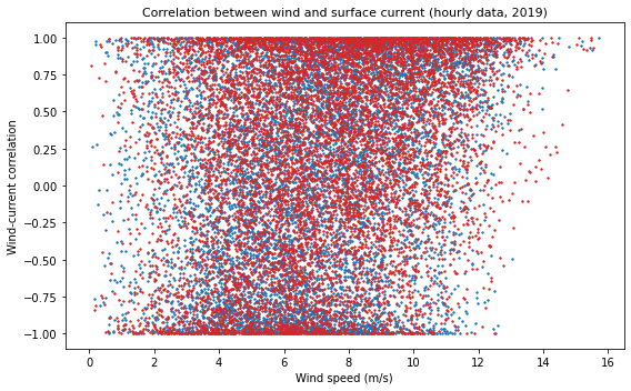
Let’s create a scatter plot to see if there is a relationship between the wind and currents.

fig, ax1 = plt.subplots()
fig.set_size_inches(8, 5)

ax1.set_xlabel('Wind speed (m/s)')
ax1.set_ylabel('Wind-current correlation')

ax1.scatter(myrmidon["windmag"], myrmidon["windcurrentcorr"], color='tab:blue', s=2) 
ax1.scatter(davies["windmag"], davies["windcurrentcorr"], color='tab:red', s=2) 

plt.title('Correlation between wind and surface current (hourly data, 2019)',fontsize=11)
fig.tight_layout()

# plt.savefig("CorrelationWindCurrent.png",dpi=300)
plt.show()
fig.clear()
plt.close(fig)
plt.clf()

<Figure size 432x288 with 0 Axes>

This scatter plot shows that the relationship between wind and current is weak. This is not surprising given that we are considering just the hourly samples, with no consideration for how long the wind has been blowing. At low wind conditions the current has an even chance of being aligned with the wind (correlation = 1) as in the opposite direction (correlation = -1), however in high wind we can see that there is much more chance that the currents are aligned with the wind.

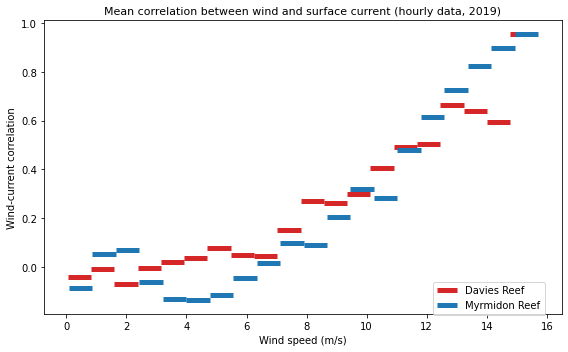
To understand this relationship better we want to understand how much the wind nudges the current in its direction. If we bin the wind speeds then collect all the correlation samples in each bin then we can see if they average to zero (indicating that there is no relationship between the wind and current) or there is average alignment.

fig, ax1 = plt.subplots()
fig.set_size_inches(8, 5)

ax1.set_xlabel('Wind speed (m/s)')
ax1.set_ylabel('Wind-current correlation')

wind = davies["windmag"]
current = davies["windcurrentcorr"]
bin_means, bin_edges, binnumber = stats.binned_statistic(wind, current, 'mean', bins=20)
ax1.hlines(bin_means, bin_edges[:-1], bin_edges[1:], colors='tab:red', lw=5,
           label='Davies Reef')


wind = myrmidon["windmag"]
current = myrmidon["windcurrentcorr"]
bin_means, bin_edges, binnumber = stats.binned_statistic(wind, current, 'mean', bins=20)
ax1.hlines(bin_means, bin_edges[:-1], bin_edges[1:], colors='tab:blue', lw=5,
           label='Myrmidon Reef')

fig.legend(loc='lower left', bbox_to_anchor=(0.75, 0.1))
plt.title('Mean correlation between wind and surface current (hourly data, 2019)',fontsize=11)
fig.tight_layout()

plt.show()
fig.clear()
plt.close(fig)
plt.clf()

<Figure size 432x288 with 0 Axes>

From this we can see that for wind speeds below 8 m/s the surface current direction is unrelated to the wind. Above this wind speed the surface current is increasingly determined by the direction of the wind. By the time the wind is 16 m/s the direction of the surface current is dominated by the wind direction.

Note: It should be remembered that this analysis is based on the eReefs Hydrodynamic model and as such is not based on real data. The eReefs model has however been tuned to accurately capture the flow dynamics of the GBR and so we would expect the estimates from this analysis to be approximately correct.

Environmental Simulation Modelling