Pandas Fundamentals
This material is adapted from the Earth and Environmental Data Science, from Ryan Abernathey (Columbia University).
import pandas as pd
import numpy as np

from matplotlib import pyplot as plt
# %config InlineBackend.figure_format = 'retina'
plt.ion()  # To trigger the interactive inline mode
Pandas Data Structures: Series
A Series represents a one-dimensional array of data. The main difference between a Series and numpy array is that a Series has an index. The index contains the labels that we use to access the data.
There are many ways to create a Series. We will just show a few.
names = ['Yasi', 'Debbie', 'Yasa']
values = [5., 4., 5.]
cyclones = pd.Series(values, index=names)
cyclones
Yasi      5.0
Debbie    4.0
Yasa      5.0
dtype: float64
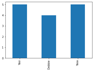
Series have built in plotting methods.
cyclones.plot(kind='bar')
<AxesSubplot:>
Arithmetic operations and most numpy function can be applied to Series. An important point is that the Series keep their index during such operations.
np.log(cyclones) / cyclones**2
Yasi      0.064378
Debbie    0.086643
Yasa      0.064378
dtype: float64
We can access the underlying index object if we need to:
cyclones.index
Index(['Yasi', 'Debbie', 'Yasa'], dtype='object')
Indexing
We can get values back out using the index via the .loc attribute
cyclones.loc['Debbie']
4.0
Or by raw position using .iloc
cyclones.iloc[1]
4.0
We can pass a list or array to loc to get multiple rows back:
cyclones.loc[['Debbie', 'Yasa']]
Debbie    4.0
Yasa      5.0
dtype: float64
And we can even use slice notation
cyclones.loc['Debbie':'Yasa']
Debbie    4.0
Yasa      5.0
dtype: float64
cyclones.iloc[:2]
Yasi      5.0
Debbie    4.0
dtype: float64
If we need to, we can always get the raw data back out as well
cyclones.values # a numpy array
array([5., 4., 5.])
cyclones.index # a pandas Index object
Index(['Yasi', 'Debbie', 'Yasa'], dtype='object')
Pandas Data Structures: DataFrame
There is a lot more to Series, but they are limit to a single “column”. A more useful Pandas data structure is the DataFrame. A DataFrame is basically a bunch of series that share the same index. It’s a lot like a table in a spreadsheet.
Below we create a DataFrame.
# first we create a dictionary
data = {'category': [5, 4, 5],
        'windspeed': [250., 215., 260.],
        'fatalities': [1, 14, 4]}
df = pd.DataFrame(data, index=['Yasi', 'Debbie', 'Yasa'])
df
| category | windspeed | fatalities | |
|---|---|---|---|
| Yasi | 5 | 250.0 | 1 |
| Debbie | 4 | 215.0 | 14 |
| Yasa | 5 | 260.0 | 4 |
Pandas handles missing data very elegantly, keeping track of it through all calculations.
df.info()
<class 'pandas.core.frame.DataFrame'>
Index: 3 entries, Yasi to Yasa
Data columns (total 3 columns):
 #   Column      Non-Null Count  Dtype
---  ------      --------------  -----
 0   category    3 non-null      int64
 1   windspeed   3 non-null      float64
 2   fatalities  3 non-null      int64
dtypes: float64(1), int64(2)
memory usage: 96.0+ bytes
A wide range of statistical functions are available on both Series and DataFrames.
df.min()
category        4.0
windspeed     215.0
fatalities      1.0
dtype: float64
df.mean()
category        4.666667
windspeed     241.666667
fatalities      6.333333
dtype: float64
df.std()
category       0.577350
windspeed     23.629078
fatalities     6.806859
dtype: float64
df.describe()
| category | windspeed | fatalities | |
|---|---|---|---|
| count | 3.000000 | 3.000000 | 3.000000 |
| mean | 4.666667 | 241.666667 | 6.333333 |
| std | 0.577350 | 23.629078 | 6.806859 |
| min | 4.000000 | 215.000000 | 1.000000 |
| 25% | 4.500000 | 232.500000 | 2.500000 |
| 50% | 5.000000 | 250.000000 | 4.000000 |
| 75% | 5.000000 | 255.000000 | 9.000000 |
| max | 5.000000 | 260.000000 | 14.000000 |
We can get a single column as a Series using python’s getitem syntax on the DataFrame object.
df['windspeed']
Yasi      250.0
Debbie    215.0
Yasa      260.0
Name: windspeed, dtype: float64
…or using attribute syntax.
df.windspeed
Yasi      250.0
Debbie    215.0
Yasa      260.0
Name: windspeed, dtype: float64
Indexing works very similar to series
df.loc['Debbie']
category        4.0
windspeed     215.0
fatalities     14.0
Name: Debbie, dtype: float64
df.iloc[1]
category        4.0
windspeed     215.0
fatalities     14.0
Name: Debbie, dtype: float64
But we can also specify the column we want to access
df.loc['Debbie', 'fatalities']
14
df.iloc[:2, 2]
Yasi       1
Debbie    14
Name: fatalities, dtype: int64
If we make a calculation using columns from the DataFrame, it will keep the same index:
df.windspeed / df.category
Yasi      50.00
Debbie    53.75
Yasa      52.00
dtype: float64
Which we can easily add as another column to the DataFrame:
df['ratio'] = df.windspeed / df.category
df
| category | windspeed | fatalities | ratio | |
|---|---|---|---|---|
| Yasi | 5 | 250.0 | 1 | 50.00 |
| Debbie | 4 | 215.0 | 14 | 53.75 |
| Yasa | 5 | 260.0 | 4 | 52.00 |
Merging Data
Pandas supports a wide range of methods for merging different datasets. These are described extensively in the documentation. Here we just give a few examples.
cyclone = pd.Series(['$246.7 M', None, '$2.73 B', '$3.6 B'],
                     index=['Yasa', 'Tino', 'Debbie', 'Yasi'],
                     name='cost')
cyclone
Yasa      $246.7 M
Tino          None
Debbie     $2.73 B
Yasi        $3.6 B
Name: cost, dtype: object
# returns a new DataFrame
df.join(cyclone)
| category | windspeed | fatalities | ratio | cost | |
|---|---|---|---|---|---|
| Yasi | 5 | 250.0 | 1 | 50.00 | $3.6 B |
| Debbie | 4 | 215.0 | 14 | 53.75 | $2.73 B |
| Yasa | 5 | 260.0 | 4 | 52.00 | $246.7 M |
# returns a new DataFrame
df.join(cyclone, how='right')
| category | windspeed | fatalities | ratio | cost | |
|---|---|---|---|---|---|
| Yasa | 5.0 | 260.0 | 4.0 | 52.00 | $246.7 M |
| Tino | NaN | NaN | NaN | NaN | None |
| Debbie | 4.0 | 215.0 | 14.0 | 53.75 | $2.73 B |
| Yasi | 5.0 | 250.0 | 1.0 | 50.00 | $3.6 B |
# returns a new DataFrame
cyc = df.reindex(['Yasa', 'Tino', 'Debbie', 'Yasi', 'Tracy'])
cyc
| category | windspeed | fatalities | ratio | |
|---|---|---|---|---|
| Yasa | 5.0 | 260.0 | 4.0 | 52.00 |
| Tino | NaN | NaN | NaN | NaN |
| Debbie | 4.0 | 215.0 | 14.0 | 53.75 |
| Yasi | 5.0 | 250.0 | 1.0 | 50.00 |
| Tracy | NaN | NaN | NaN | NaN |
We can also index using a boolean series. This is very useful
huge = df[df.category > 4]
huge
| category | windspeed | fatalities | ratio | |
|---|---|---|---|---|
| Yasi | 5 | 250.0 | 1 | 50.0 |
| Yasa | 5 | 260.0 | 4 | 52.0 |
df['is_huge'] = df.category > 4
df
| category | windspeed | fatalities | ratio | is_huge | |
|---|---|---|---|---|---|
| Yasi | 5 | 250.0 | 1 | 50.00 | True |
| Debbie | 4 | 215.0 | 14 | 53.75 | False |
| Yasa | 5 | 260.0 | 4 | 52.00 | True |
Modifying Values
We often want to modify values in a dataframe based on some rule. To modify values, we need to use .loc or .iloc
df.loc['Debbie', 'windspeed'] = 285
df.loc['Yasa', 'category'] += 1
df
| category | windspeed | fatalities | ratio | is_huge | |
|---|---|---|---|---|---|
| Yasi | 5 | 250.0 | 1 | 50.00 | True |
| Debbie | 4 | 285.0 | 14 | 53.75 | False |
| Yasa | 6 | 260.0 | 4 | 52.00 | True |
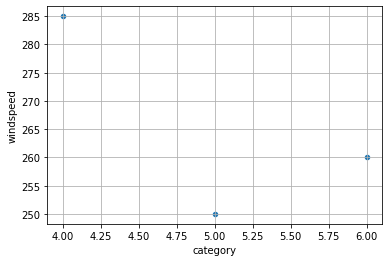
Plotting
DataFrames have all kinds of useful plotting built in.
df.plot(kind='scatter', x='category', y='windspeed', grid=True)
<AxesSubplot:xlabel='category', ylabel='windspeed'>
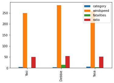
df.plot(kind='bar')
<AxesSubplot:>
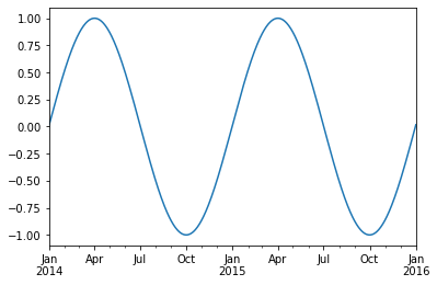
Time Indexes
Indexes are very powerful. They are a big part of why Pandas is so useful. There are different indices for different types of data. Time Indexes are especially great!
two_years = pd.date_range(start='2014-01-01', end='2016-01-01', freq='D')
timeseries = pd.Series(np.sin(2 *np.pi *two_years.dayofyear / 365),
                       index=two_years)
timeseries.plot()
<AxesSubplot:>
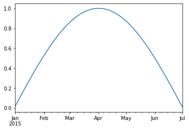
We can use python’s slicing notation inside .loc to select a date range.
timeseries.loc['2015-01-01':'2015-07-01'].plot()
<AxesSubplot:>
The TimeIndex object has lots of useful attributes
timeseries.index.month
Int64Index([ 1,  1,  1,  1,  1,  1,  1,  1,  1,  1,
            ...
            12, 12, 12, 12, 12, 12, 12, 12, 12,  1],
           dtype='int64', length=731)
timeseries.index.day
Int64Index([ 1,  2,  3,  4,  5,  6,  7,  8,  9, 10,
            ...
            23, 24, 25, 26, 27, 28, 29, 30, 31,  1],
           dtype='int64', length=731)
Reading Data Files
In this example, we will use the eReefs Extraction tool from AIMS and look at Davies Reef which is located at 18.8S/147.6E.
The CSV file was downloaded from the AIMS extraction tool with the following settings:
Data collection: GBR1 Hydro (Version 2)
Variables: Eastward wind speed (wspeed_u), Northward wind speed (wspeed_v), Northward current (v), Eastward current (u)
Date range: 2010-2021
Time step: hourly Depths: -2.35 m
Once the extraction request was submitted the dataset was created after an one hour of processing the data was available for download from Extraction request: Example dataset: Wind-vs-Current at Davies and Myrmidon Reefs (2019).
After download we have a file called DaviesReef_timeseries.csv.
Tip
To read it into pandas, we will use the read_csv function. This function is incredibly complex and powerful. You can use it to extract data from almost any text file. However, you need to understand how to use its various options.
With no options, this is what we get.
df = pd.read_csv('examples/DaviesReef_timeseries.csv')
df.head()
| date current wind salinity temperature | |
|---|---|
| 0 | 2010-09-01 0.18839505 7.481102 35.47361 25.17717 |
| 1 | 2010-09-02 0.28618774 4.9959917 35.48525 25.26... |
| 2 | 2010-09-03 0.29367417 6.024843 35.462696 25.20... |
| 3 | 2010-09-04 0.28546846 5.7049136 35.44163 25.38... |
| 4 | 2010-09-05 0.34016508 4.3658934 35.41293 25.7196 |
Pandas failed to identify the different columns. This is because it was expecting standard CSV (comma-separated values) file. In our file, instead, the values are separated by whitespace. And not a single whilespace–the amount of whitespace between values varies. We can tell pandas this using the sep keyword.
df = pd.read_csv('examples/DaviesReef_timeseries.csv', sep='\s+')
df.head()
| date | current | wind | salinity | temperature | |
|---|---|---|---|---|---|
| 0 | 2010-09-01 | 0.188395 | 7.481102 | 35.473610 | 25.177170 |
| 1 | 2010-09-02 | 0.286188 | 4.995992 | 35.485250 | 25.262072 |
| 2 | 2010-09-03 | 0.293674 | 6.024843 | 35.462696 | 25.201515 |
| 3 | 2010-09-04 | 0.285468 | 5.704914 | 35.441630 | 25.385157 |
| 4 | 2010-09-05 | 0.340165 | 4.365893 | 35.412930 | 25.719600 |
Great! It worked.
Often missing values are set either to -9999 or -99. Let’s tell this to pandas by assigning nan to these specific values.
df = pd.read_csv('examples/DaviesReef_timeseries.csv', sep='\s+', na_values=[-9999.0, -99.0])
df.head()
| date | current | wind | salinity | temperature | |
|---|---|---|---|---|---|
| 0 | 2010-09-01 | 0.188395 | 7.481102 | 35.473610 | 25.177170 |
| 1 | 2010-09-02 | 0.286188 | 4.995992 | 35.485250 | 25.262072 |
| 2 | 2010-09-03 | 0.293674 | 6.024843 | 35.462696 | 25.201515 |
| 3 | 2010-09-04 | 0.285468 | 5.704914 | 35.441630 | 25.385157 |
| 4 | 2010-09-05 | 0.340165 | 4.365893 | 35.412930 | 25.719600 |
Great. The missing data is now represented by NaN.
What data types did pandas infer?
df.info()
<class 'pandas.core.frame.DataFrame'>
RangeIndex: 3815 entries, 0 to 3814
Data columns (total 5 columns):
 #   Column       Non-Null Count  Dtype
---  ------       --------------  -----
 0   date         3815 non-null   object
 1   current      3815 non-null   float64
 2   wind         3815 non-null   float64
 3   salinity     3815 non-null   float64
 4   temperature  3815 non-null   float64
dtypes: float64(4), object(1)
memory usage: 149.1+ KB
One problem here is that Pandas did not recognize the date column as a date. Let’s help it.
df = pd.read_csv('examples/DaviesReef_timeseries.csv', sep='\s+',
                 na_values=[-9999.0, -99.0],
                 parse_dates=['date'])
df.info()
<class 'pandas.core.frame.DataFrame'>
RangeIndex: 3815 entries, 0 to 3814
Data columns (total 5 columns):
 #   Column       Non-Null Count  Dtype
---  ------       --------------  -----
 0   date         3815 non-null   datetime64[ns]
 1   current      3815 non-null   float64
 2   wind         3815 non-null   float64
 3   salinity     3815 non-null   float64
 4   temperature  3815 non-null   float64
dtypes: datetime64[ns](1), float64(4)
memory usage: 149.1 KB
It worked! Finally, let’s tell pandas to use the date column as the index.
df = df.set_index('date')
df.head()
| current | wind | salinity | temperature | |
|---|---|---|---|---|
| date | ||||
| 2010-09-01 | 0.188395 | 7.481102 | 35.473610 | 25.177170 |
| 2010-09-02 | 0.286188 | 4.995992 | 35.485250 | 25.262072 |
| 2010-09-03 | 0.293674 | 6.024843 | 35.462696 | 25.201515 |
| 2010-09-04 | 0.285468 | 5.704914 | 35.441630 | 25.385157 |
| 2010-09-05 | 0.340165 | 4.365893 | 35.412930 | 25.719600 |
We can now access values by time:
df.loc['2014-08-07']
current         0.381858
wind           11.198019
salinity       35.307660
temperature    23.866120
Name: 2014-08-07 00:00:00, dtype: float64
Or use slicing to get a range:
df2014 = df.loc['2014-01-01':'2014-12-31']
df2016 = df.loc['2016-01-01':'2016-12-31']
df2018 = df.loc['2018-01-01':'2018-12-31']
df2020 = df.loc['2020-01-01':'2020-12-31']
df2014
| current | wind | salinity | temperature | |
|---|---|---|---|---|
| date | ||||
| 2014-01-01 | 0.400576 | 5.939211 | 35.446510 | 28.987250 |
| 2014-01-02 | 0.382042 | 3.748479 | 35.437440 | 29.117306 |
| 2014-01-03 | 0.396745 | 4.321397 | 35.470460 | 29.362583 |
| 2014-01-04 | 0.438115 | 5.537916 | 35.474777 | 29.393948 |
| 2014-01-05 | 0.440387 | 5.804630 | 35.441086 | 29.072742 |
| ... | ... | ... | ... | ... |
| 2014-12-27 | 0.229368 | 5.385712 | 35.412727 | 28.865137 |
| 2014-12-28 | 0.205974 | 3.610898 | 35.416306 | 29.263445 |
| 2014-12-29 | 0.303206 | 3.092528 | 35.432480 | 29.667050 |
| 2014-12-30 | 0.254966 | 2.479212 | 35.479332 | 30.116217 |
| 2014-12-31 | 0.285224 | 2.497501 | 35.500930 | 30.287010 |
365 rows × 4 columns
Quick Statistics
df.describe()
| current | wind | salinity | temperature | |
|---|---|---|---|---|
| count | 3815.000000 | 3815.000000 | 3815.000000 | 3815.000000 |
| mean | 0.265826 | 6.708479 | 35.182442 | 26.610127 |
| std | 0.084196 | 2.643628 | 0.292870 | 1.936466 |
| min | 0.061780 | 1.245048 | 32.956253 | 22.933332 |
| 25% | 0.209833 | 4.613128 | 35.042687 | 24.853140 |
| 50% | 0.256591 | 6.528472 | 35.263058 | 26.700006 |
| 75% | 0.308909 | 8.581003 | 35.375860 | 28.180752 |
| max | 0.817050 | 18.900612 | 35.763687 | 31.598990 |
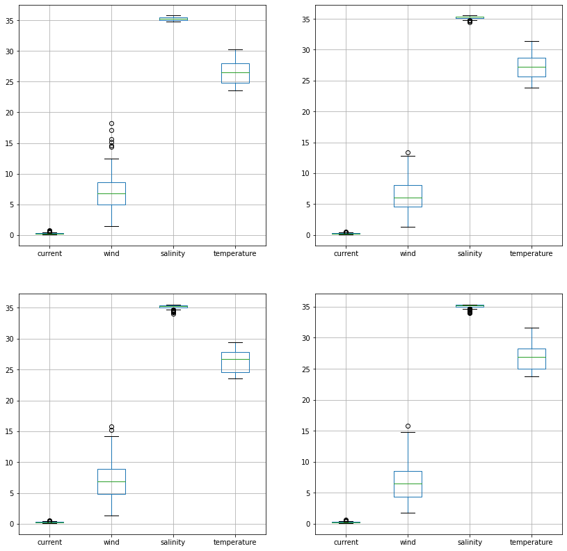
Plotting Values
We can now quickly make plots of the data
fig, ax = plt.subplots(ncols=2, nrows=2, figsize=(14,14))

df2014.iloc[:, :].boxplot(ax=ax[0,0])
df2016.iloc[:, :].boxplot(ax=ax[0,1])
df2018.iloc[:, :].boxplot(ax=ax[1,0])
df2020.iloc[:, :].boxplot(ax=ax[1,1])
<AxesSubplot:>
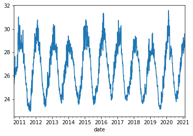
Pandas is very “time aware”:
df.temperature.plot()
<AxesSubplot:xlabel='date'>
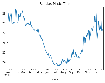
Note: we could also manually create an axis and plot into it.
fig, ax = plt.subplots()
df2018.temperature.plot(ax=ax)
ax.set_title('Pandas Made This!')
Text(0.5, 1.0, 'Pandas Made This!')
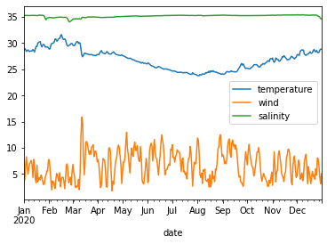
df2020[['temperature', 'wind', 'salinity']].plot()
<AxesSubplot:xlabel='date'>
Resampling
Since pandas understands time, we can use it to do resampling.
# monthly reampler object
rs_obj = df.resample('MS')
rs_obj
<pandas.core.resample.DatetimeIndexResampler object at 0x7fb2ce581d30>
rs_obj.mean()
| current | wind | salinity | temperature | |
|---|---|---|---|---|
| date | ||||
| 2010-09-01 | 0.281347 | 5.869099 | 35.365671 | 26.017173 |
| 2010-10-01 | 0.283938 | 8.118046 | 35.368278 | 26.372507 |
| 2010-11-01 | 0.268329 | 7.007014 | 35.384552 | 26.872662 |
| 2010-12-01 | 0.342128 | 5.501357 | 35.019846 | 29.165949 |
| 2011-01-01 | 0.306163 | 5.960649 | 34.620039 | 29.236425 |
| ... | ... | ... | ... | ... |
| 2020-10-01 | 0.257407 | 6.045590 | 35.242590 | 25.873325 |
| 2020-11-01 | 0.268678 | 6.381081 | 35.325458 | 27.001825 |
| 2020-12-01 | 0.288298 | 5.469824 | 35.251699 | 28.221937 |
| 2021-01-01 | 0.289114 | 7.052687 | 34.391954 | 28.522526 |
| 2021-02-01 | 0.236967 | 3.992934 | 34.692678 | 29.264261 |
126 rows × 4 columns
We can chain all of that together
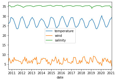
df_mm = df.resample('MS').mean()
df_mm[['temperature', 'wind', 'salinity']].plot()
<AxesSubplot:xlabel='date'>
Next notebook, we will dig deeper into resampling, rolling means, and grouping operations (groupby).