Introduction to numpy
This material is adapted from the Earth and Environmental Data Science and the Scientific Programming course from Fabien Maussion.
You might have read somewhere that Python is “slow” in comparison to some other languages. While generally true, this statement has only little meaning without context. As a scripting language (e.g. simplify tasks such as file renaming, data download, etc.), python is fast enough. For numerical computations (like the computations done by a regional wave model like SHOC or by a machine learning algorithm), “pure” Python is very slow indeed. Fortunately, there is a way to overcome this problem!
In this notebook, we are going to explain why the numpy library was created.
Note
Python Versions Numpy is the fundamental library which transformed the general purpose Python language into a scientific language like Matlab, R or IDL.
Numpy
Why is numpy so much faster than pure python? One of the major reasons is vectorization, which is the process of applying mathematical operations to all elements of an array (“vector”) at once instead of looping through them like we would do in pure python. for loops in Python are slow because for each addition, python has to:
access the elements a and b in the lists A and B
check the type of both a and b
apply the
+operator on the data they storestore the result.
Numpy skips the first two steps and does them only once before the actual operation. What does numpy know about the addition operation that the pure python version can’t infer?
the type of all numbers to add
the type of the output
the size of the output array (same as input)
Numpy can use this information to optimize the computation, but this isn’t possible without trade-offs. See the following for example:
import numpy as np
What did we just do? We imported the numpy package and we renamed it to np for efficiency. It must now be referenced as np within our notebook, or it will not be recognized.
This brings new variables (mostly functions and instances) into our interpreter. We access them by pressing np. in the cell below:
np.
Numpy Documentation
The numpy documentation is crucial and can be found here.
I’ll be honest: without an internet connection, I am a very bad Python programmer. I don’t expect you to learn all the python commands by heart. Similarly, I encourage you to use the internet to find help during your project.
However, there is a difference between “getting help to find how to realize a specific task” and “asking for someone to do the project for you”. The border line between the two might be subtle, but I’m sure you’ll know when you cross it: at the moment you stopped using your brain and simply copy/pasted code from one site to your assignment script, you crossed it.
Anatomy of a ndarray
From the numpy reference:
N-dimensional ndarray’s are the core structure of the numpy library. It is a multidimensional container of items of the same type and size. The number of dimensions and items in an array is defined by its shape, which is a tuple of N positive integers that specify the number of items in each dimension. The type of items in the array is specified by a separate data-type object (dtype), one of which is associated with each ndarray.
All ndarrays are homogenous: every item takes up the same size block of memory, and all blocks are interpreted in exactly the same way.
An item extracted from an array, e.g., by indexing, is represented by a Python object whose type is one of the array scalar types built in NumPy.
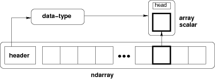
Fig. 7 Conceptual diagram showing the relationship between the three fundamental objects used to describe the data in an array: 1) the ndarray itself, 2) the data-type object that describes the layout of a single fixed-size element of the array, 3) the array-scalar Python object that is returned when a single element of the array is accessed.
Figure:
import numpy as np
x = np.array([[1, 2, 3], [4, 5, 6]], int)
type(x)
numpy.ndarray
x.dtype # x is of type ndarray, but the data it contains is not
dtype('int64')
Numpy was created to work with numbers, and large arrays of numbers with the same type. Some of ndarray’s attributes give us information about the memory they need:
print(x.itemsize)  # size of one element (int) in bytes
print(x.nbytes)    # size of 2 * 3 = 6 elements in bytes
8
48
The shape of an array formalizes how the data values are accessed or printed:
x.shape
(2, 3)
What is the shape?
type(a.shape)
---------------------------------------------------------------------------
NameError                                 Traceback (most recent call last)
<ipython-input-7-d54d54d1481c> in <module>
----> 1 type(a.shape)

NameError: name 'a' is not defined
print(x)
[[1 2 3]
 [4 5 6]]
However, the data is one-dimensional and contiguous in memory. I.e. the 1D segment of computer memory stored by the array is combined with an indexing scheme that maps N-dimensional indexes into the location of an item in the block. Concretely, this means that there is no difference in the memory layout of these two arrays:
a = np.arange(9)
b = a.reshape((3, 3))  # what does "reshape" do?
Both are internally stored using a one dimensional memory block. The difference lies in the way numpy gives access to the internal data:
a[4], b[1, 1]
(4, 4)
This means that elementwise operations have the same execution speed for N dimensional arrays as for 1-D arrays. Now, let’s replace an element from array b:
b[1, 1] = 99
b
array([[ 0,  1,  2],
       [ 3, 99,  5],
       [ 6,  7,  8]])
Since the indexing [1, 1] is on the left-hand side of the assignment operator, we modified b in-place. Numpy located the block of memory that needed to be changed and replaced it with another number. Since all these numbers are integers with a fixed memory size, this is not a problem. But what happens if we try to assign another data type?
b[1, 1] = 999.99
b
array([[  0,   1,   2],
       [  3, 999,   5],
       [  6,   7,   8]])
The float is converted to an integer!
Warning
This is a dangerous “feature” of numpy and should be used with care.
Another extremely important mechanism of ndarrays is their internal handling of data. Indeed:
a
array([ 0, 1, 2, 3, 999, 5, 6, 7, 8])
What happened here? Modifying the data in b also modified the data in a! More precisely, both arrays share the same internal data: b is a view of the data owned by a.
b.base is a
True
a.base is None
True
np.shares_memory(a, b)
True
This allows for memory efficient reshaping and vector operations on numpy arrays, but is a source of confusion for many. in this lecture, we will look into more detail which operations return a view and which return a copy.
Warning
The concept of views and copies of ndarray is central to numpy. Make sure you understood the examples above well before going on.
Creating ndarrays
There are many ways to create numpy arrays. The functions you will use most often are:
np.emtpy, np.zeros, np.ones, np.full
These three work the same way, The first argument defines the shape of the array:
a = np.ones((2, 3, 4))
a
array([[[1., 1., 1., 1.],
        [1., 1., 1., 1.],
        [1., 1., 1., 1.]],

       [[1., 1., 1., 1.],
        [1., 1., 1., 1.],
        [1., 1., 1., 1.]]])
The dtype kwarg specifies the type:
np.zeros(2, dtype=bool)
array([False, False])
a = np.empty((2, 3), dtype=np.float32)
a.dtype
dtype('float32')
What is an “empty” array by the way?
a
array([[2.3694278e-38, 2.3694278e-38, 2.3694278e-38],
       [2.3694278e-38, 2.3694278e-38, 2.3694278e-38]], dtype=float32)
What are all these numbers? As it turns out, they are completely unpredictable: with np.empty, numpy just takes a free slot of memory somewhere, and doesn’t change the bits in it. Computers are smart enough: when deleting a variable, they are just removing the pointer (the address) to this series of bits, not deleting them (this would cost too much time).
Tip
By the way The same is true for the “delete” function in your operating system by the way: even after “deleting” a file, be aware that a motivated hacker can find and recover your data (data-recovery).
So, why using np.empty instead of np.zeros? Mostly for performance reasons. With np.empty, numpy spares the step of setting all the underlying bits to zero:
%timeit np.empty(2000)
747 ns ± 30 ns per loop (mean ± std. dev. of 7 runs, 1000000 loops each)
%timeit np.ones(2000)
3.49 µs ± 63.1 ns per loop (mean ± std. dev. of 7 runs, 100000 loops each)
So at least a factor 10 faster on my laptop. If you know that your are going to use your array as data storage and fill it later on, it might be a good idea to use np.empty. In practice, however, performance doesn’t matter that much and avoiding bugs is more important: initialize your arrays with NaNs (Not a Number) in order to easily find out if all values were actually set by your program after completion:
np.full((2, 3), np.NaN)
array([[nan, nan, nan],
       [nan, nan, nan]])
np.array
np.array converts existing data to a ndarray:
np.array([[1, 2, 3], [4, 5, 6]], float)
array([[1., 2., 3.],
       [4., 5., 6.]])
np.copy
When a variable is assigned to another variable in Python, it creates a new reference to the object it contains, NOT a copy:
a = np.zeros(3)
b = a
b[1] = 1
a  # ups, didn't want to do that!
array([0., 1., 0.])
This behavior is not specific to numpy, but to python itself. Remember? Can you predict the outcome of the following code:
a = [1, 2, 3]
b = a
b.append(4)
print(a)
If you learned programming with another language (Matlab, R, C), compare this behavior to the language you used before.
This is why np.copy is useful:
a = np.zeros(3)
b = a.copy()  # same as np.copy(a)
b[1] = 1
a  # ah!
array([0., 0., 0.])
np.arange
np.arange(10)
array([0, 1, 2, 3, 4, 5, 6, 7, 8, 9])
Be careful! the start and stop arguments define the half open interval [start, stop[:
np.arange(3, 15, 3)
array([ 3, 6, 9, 12])
np.arange(3, 15.00000001, 3)
array([ 3., 6., 9., 12., 15.])
np.linspace
Regularly spaced intervals between two values (both limits are included this time):
np.linspace(0, 1, 11)
array([0. , 0.1, 0.2, 0.3, 0.4, 0.5, 0.6, 0.7, 0.8, 0.9, 1. ])
The shape of ndarrays
Is numpy row-major or column-major order?
The default order in numpy is that of the C-language: row-major. This means that the array:
a = np.array([[1, 2, 3],
              [4, 5, 6]])
a
array([[1, 2, 3],
       [4, 5, 6]])
has two rows and three columns, the rows being listed first:
a.shape
(2, 3)
and that the internal representation in memory is sorted by rows:
a.flatten()
array([1, 2, 3, 4, 5, 6])
A consequence is that reading data out of rows (first dimension in the array) is usually a bit faster than reading out of columns:
t = np.zeros((1000, 1000))
%timeit t[[0], :]
%timeit t[:, [0]]
2.85 µs ± 24.7 ns per loop (mean ± std. dev. of 7 runs, 100000 loops each)
4.43 µs ± 57.8 ns per loop (mean ± std. dev. of 7 runs, 100000 loops each)
This is different from some other languages like FORTRAN, Matlab, R, or IDL. In my opinion though, most of the time it doesn’t matter much to remember whether it is row- or column-major, as long as you remember which dimension is what. Still, this can be a source of confusion at first, especially if you come from one of these column-major languages.
Most datasets are then going to store the data in a way that allows faster retrieval along the dimension which is read most often: for environmental datasets, this is often going to be the “time” dimension, i.e. the size of the time dimension is going to give the size of array.shape[0].
My personal way to deal with this when I started using numpy is that I always thought of numpy being in the “wrong” order. If you have data defined in four dimensions (x, y, z, t in the “intuitive”, mathematical order), then it is often stored in numpy with the shape (t, z, y, x).
The 4D arrays that we will use a lot in the course are stored on disk as netCDF files, and their description read something like:
	double t(time, zc, latitude, longitude) ;
		t:units = "degrees C" ;
		t:long_name = "Temperature" ;
which is also the order used by numpy:
# you can't do this at home!
input_AIMS = "http://thredds.ereefs.aims.gov.au/thredds/dodsC/s3://aims-ereefs-public-prod/derived/ncaggregate/ereefs/gbr4_v2/daily-monthly/EREEFS_AIMS-CSIRO_gbr4_v2_hydro_daily-monthly-2020-03.nc"

import netCDF4 as nc

nc_data = nc.Dataset(input_AIMS, 'r')

temp = nc_data.variables['temp']
temp.coordinates,temp.shape
('time zc latitude longitude', (31, 17, 723, 491))
temp[0,:,:,:]
masked_array(
  data=[[[      nan,       nan,       nan, ...,       nan,       nan,
                nan],
         [      nan,       nan,       nan, ..., 19.424944, 19.453869,
          19.533148],
         [      nan,       nan,       nan, ..., 19.306637, 19.453146,
          19.526852],
         ...,
         [      nan,       nan,       nan, ...,       nan,       nan,
                nan],
         [      nan,       nan,       nan, ...,       nan,       nan,
                nan],
         [      nan,       nan,       nan, ...,       nan,       nan,
                nan]],

        [[      nan,       nan,       nan, ...,       nan,       nan,
                nan],
         [      nan,       nan,       nan, ..., 20.083586, 20.106384,
          20.165667],
         [      nan,       nan,       nan, ..., 19.98137 , 20.104473,
          20.151701],
         ...,
         [      nan,       nan,       nan, ...,       nan,       nan,
                nan],
         [      nan,       nan,       nan, ...,       nan,       nan,
                nan],
         [      nan,       nan,       nan, ...,       nan,       nan,
                nan]],

        [[      nan,       nan,       nan, ...,       nan,       nan,
                nan],
         [      nan,       nan,       nan, ..., 20.611938, 20.625534,
          20.657   ],
         [      nan,       nan,       nan, ..., 20.528597, 20.617815,
          20.627022],
         ...,
         [      nan,       nan,       nan, ...,       nan,       nan,
                nan],
         [      nan,       nan,       nan, ...,       nan,       nan,
                nan],
         [      nan,       nan,       nan, ...,       nan,       nan,
                nan]],

        ...,

        [[      nan,       nan,       nan, ...,       nan,       nan,
                nan],
         [      nan,       nan,       nan, ..., 25.970568, 25.960426,
          25.930021],
         [      nan,       nan,       nan, ..., 25.998253, 25.957634,
          25.917608],
         ...,
         [      nan,       nan,       nan, ...,       nan,       nan,
                nan],
         [      nan,       nan,       nan, ...,       nan,       nan,
                nan],
         [      nan,       nan,       nan, ...,       nan,       nan,
                nan]],

        [[      nan,       nan,       nan, ...,       nan,       nan,
                nan],
         [      nan,       nan,       nan, ..., 26.114777, 26.100243,
          26.058285],
         [      nan,       nan,       nan, ..., 26.157967, 26.097944,
          26.034834],
         ...,
         [      nan,       nan,       nan, ...,       nan,       nan,
                nan],
         [      nan,       nan,       nan, ...,       nan,       nan,
                nan],
         [      nan,       nan,       nan, ...,       nan,       nan,
                nan]],

        [[      nan,       nan,       nan, ...,       nan,       nan,
                nan],
         [      nan,       nan,       nan, ..., 26.177057, 26.161913,
          26.117983],
         [      nan,       nan,       nan, ..., 26.22213 , 26.159912,
          26.09275 ],
         ...,
         [      nan,       nan,       nan, ...,       nan,       nan,
                nan],
         [      nan,       nan,       nan, ...,       nan,       nan,
                nan],
         [      nan,       nan,       nan, ...,       nan,       nan,
                nan]]],
  mask=False,
  fill_value=1e+20,
  dtype=float32)
This order might be different in other languages. It’s just a convention!
Tip
Anyways, with some experience you’ll see that there is always a way to get numpy arrays in the shape you want them. It is sometimes going to be confusing and you are going to need some googling skills, but you’ll manage. All the tools at your disposition for these purposes are listed in the array manipulation documentation page.
Parenthesis: note that numpy also allows to use the column-major order you may be familiar with:
a = np.array([[1, 2, 3],
              [4, 5, 6]])
a.flatten(order='F')
array([1, 4, 2, 5, 3, 6])
I do not recommend to take this path unless really necessary: sooner or later you are going to regret it. If you really need to flatten an array this way, I recommend the more numpy-like:
a.T.flatten()
array([1, 4, 2, 5, 3, 6])
Indexing
Indexing refers to the act of accessing values in an array by their index, i.e. their position in the array.
There are many ways to index arrays, and the numpy documentation about the subject is excellent. Here we will just revise some of the most important aspects of it.
Get some individual elements of x
x = np.array([0, 1, 2, 3, 4, 5, 6, 7, 8, 9])
x[0],x[-1]
(0, 9)
Slicing
The common way to do slicing is by using the following syntax:
x[1:7:2]
array([1, 3, 5])
The start:stop:step syntax is actually creating a python slice object. The statement above is therefore the literal version of the less concise:
x[slice(1, 7, 2)]
array([1, 3, 5])
The step can be used to reverse (flip) the order of elements in an array:
x[::-1]
array([9, 8, 7, 6, 5, 4, 3, 2, 1, 0])
Inverting the elements that way is very fast. It is not significantly slower than reading the data in order:
%timeit x[::-1]
219 ns ± 2.36 ns per loop (mean ± std. dev. of 7 runs, 1000000 loops each)
%timeit x[::1]
202 ns ± 4.15 ns per loop (mean ± std. dev. of 7 runs, 1000000 loops each)
How can that be? Again, it has something to do with the internal memory layout of an array. Slicing always returns a view of an array. That is:
x = np.array([0, 1, 2, 3, 4, 5, 6, 7, 8, 9], dtype=float)
y = x[::-1]
y[0] = np.NaN
x  # ups, I also changed x, but at position 9!
array([ 0., 1., 2., 3., 4., 5., 6., 7., 8., nan])
Or:
x = np.array([0, 1, 2, 3, 4, 5, 6, 7, 8, 9], dtype=float)
y = x[2:4]
y[0] = np.NaN
x  # ups, I also changed x, but at position 2!
array([ 0., 1., nan, 3., 4., 5., 6., 7., 8., 9.])
It is very important to keep the view mechanism in mind when writing numpy code. It is a great advantage for performance considerations, but it might lead to unexpected results if you are not careful!
Integer indexing
Integer indexing happens when selecting data points based on their coordinates:
x = np.array([[1, 2, 3],
              [4, 5, 6]])

x[[0, 1, 1], [0, 2, 0]]
array([1, 6, 4])
Let’s try to get the corner elements of a 4x3 array:
x = np.array([[ 0,  1,  2],
              [ 3,  4,  5],
              [ 6,  7,  8],
              [ 9, 10, 11]])
ycoords = [0, 0, 3, 3]
xcoords = [0, 2, 0, 2]
x[ycoords, xcoords]
array([ 0, 2, 9, 11])
It may be easier for you to see the indexing command as such: we are indexing the array at 4 locations: (0, 0), (0, 2), (3, 0) and (3, 2). Therefore, the output array is of length 4 and keeps the order of the coordinate points of course.
A useful feature of advanced indexing is that the shape of the indexers is conserved by the output:
ycoords = [[0 ,  0],
           [-1, -1]]
xcoords = [[ 0, -1],
           [ 0, -1]]
x[ycoords, xcoords]
array([[ 0,  2],
       [ 9, 11]])
Unlike basic indexing, integer indexing doesn’t return a view. We have two ways to test if this is the case:
x = np.array([1, 2, 3, 4])
y = x[[1, 3]]
y.base is x  # y doesn't share memory with x
False
y[0] = 999  # changing y doesn't alter x
x
array([1, 2, 3, 4])
Boolean indexing: indexing based on a condition
Instead of integers, booleans can be used for indexing:
a = np.array([1, 2, 3, 4])
a[[True,  False, True, False]]
array([1, 3])
Unlike integer-based indexing, the shape of the indexer and the array must match (except when broadcasting occurs, see below).
The most frequent application of boolean indexing is to select values based on a condition:
x = np.array([[ 0,  1,  2],
              [ 3,  4,  5],
              [ 6,  7,  8],
              [ 9, 10, 11]])
x[x >= 8]
array([ 8, 9, 10, 11])
What is the shape of x >= 8? Try it! And try another command, too: ~ (x >= 8).
As you can see, boolean indexing in this case returns a 1D array of the same length as the number of True in the indexer.
Another way to do indexing based on a condition is to use the np.nonzero function:
nz = np.nonzero(x >= 8)
nz
(array([2, 3, 3, 3]), array([2, 0, 1, 2]))
This creates a tuple object of integer arrays specifying the location of where the condition is True, thus it is directly applicable as an indexer:
x[nz]
array([ 8, 9, 10, 11])
In practice there is no difference between x[x >= 8] and x[np.nonzero(x >= 8)], but the former is faster in most cases. np.nonzero is still very useful if you want to get access to the location of where certain conditions are met in an array. Both are using advanced indexing, thus returning a copy of the array.
Universal functions
A universal function (or ufunc for short) is a function that operates on ndarrays in an element-by-element fashion. ufuncs are a core element of the numpy library, and you already used them without noticing: arithmetic operations like multiplication or addition are ufuncs, and trigonometric operations like np.sin or np.cos are ufuncs as well.
Numpy ufuncs are coded in C, which means that they can apply repeated operations on array elements much faster than their python equivalent. Numpy users use ufuncs to vectorize their code.
Note that some ufuncs are hidden from you: calling a + b on ndarrays is actually calling np.add internally. How it is possible for numpy to mess around with the Python syntax in such a way is going to be the topic of another lecture.
The numpy documentation lists all available ufuncs to date. Have a quick look at them, just to see how many there are!
Broadcasting
Copyright note: much of the content of this section (including images) is copied from the EricsBroadcastingDoc page on SciPy.
When two arrays have the same shape, multiplying them using the multiply ufunc is easy:
a = np.array([1.0, 2.0, 3.0])
b = np.array([2.0, 2.0, 2.0])
If the shape of the two arrays do not match, however, numpy will raise a ValueError:
a = np.array([0.0, 10.0, 20.0, 30.0])
b = np.array([1.0, 2.0, 3.0])
a + b
---------------------------------------------------------------------------
ValueError                                Traceback (most recent call last)
<ipython-input-58-cec5b7244703> in <module>
      1 a = np.array([0.0, 10.0, 20.0, 30.0])
      2 b = np.array([1.0, 2.0, 3.0])
----> 3 a + b

ValueError: operands could not be broadcast together with shapes (4,) (3,)
But what does “could not be broadcast together” actually mean? Broadcasting is a term which is quite specific to numpy. From the documentation: “broadcasting describes how numpy treats arrays with different shapes during arithmetic operations”. In which cases does numpy allow arrays of different shape to be associated together via universal functions?
The simplest example is surely the multiplication with a scalar:
a = np.array([1, 2, 3])
b = 2.
a * b
array([2., 4., 6.])
The action of broadcasting can schematically represented as a “stretching” of the scalar so that the target array b is as large as the array a:
The rule governing whether two arrays have compatible shapes for broadcasting can be expressed in a single sentence:
The Broadcasting Rule: in order to broadcast, the size of the trailing axes for both arrays in an operation must either be the same size or one of them must be one.
For example, let’s multiply an array of shape(4, 3) with an array of shape (3) (both trailing axes are of length 3):
a = np.array([[ 0,  0,  0],
              [10, 10, 10],
              [20, 20, 20],
              [30, 30, 30]])
b = np.array([0, 1, 2])
a + b
array([[ 0,  1,  2],
       [10, 11, 12],
       [20, 21, 22],
       [30, 31, 32]])
Schematically, the array is stretched in the dimension which is missing to fill the gap between the two shapes:
Broadcasting provides a convenient way of taking the outer product (or any other outer operation) of two arrays. The following example shows an outer addition operation of two 1D arrays that produces the same result as above:
a = np.array([0,  10,  20, 30])
b = np.array([0, 1, 2])
a.reshape((4, 1)) + b
array([[ 0,  1,  2],
       [10, 11, 12],
       [20, 21, 22],
       [30, 31, 32]])
In this case, broadcasting stretches both arrays to form an output array larger than either of the initial arrays.
Note: a convenient syntax for the reshaping operation above is following:
a[..., np.newaxis]
array([[ 0],
       [10],
       [20],
       [30]])
a[..., np.newaxis].shape
(4, 1)
where np.newaxis is used to increase the dimension of the existing array by one more dimension where needed.
Broadcasting is quite useful when writing vectorized functions that apply on vectors and matrices. You will often use broadcasting when working with statistical or physical models dealing with high-dimensional arrays.
Take home points
numpy is the core library of the scientific python stack. It is used by many (many) companies and researchers worldwide, and its documentation is good. Use it! There is a user guide to get you started, but the reference is more complete.
“views” allow numpy to spare memory by giving various variables access to the same data. This is good for memory optimization, but error prone: always keep track of the variables pointing to the same data!
universal functions (“ufuncs”) is a fancy name for vectorized operations in numpy. You will see the term ufunc quite often in the documentation
using broadcasting you can operate on arrays with different shapes in a very elegant manner. The rule of broadcasting is simple: in order to broadcast, the size of the trailing axes for both arrays in an operation must either be the same size or one of them must be one.