Xarray Fundamentals
This material is adapted from the Earth and Environmental Data Science, from Ryan Abernathey (Columbia University).
Xarray data structures
Important
Like Pandas, xarray has two fundamental data structures:
a
DataArray, which holds a single multi-dimensional variable and its coordinatesa
Dataset, which holds multiple variables that potentially share the same coordinates
DataArray
A DataArray has four essential attributes:
values: anumpy.ndarrayholding the array’s valuesdims: dimension names for each axis (e.g.,('x', 'y', 'z'))coords: a dict-like container of arrays (coordinates) that label each point (e.g., 1-dimensional arrays of numbers, datetime objects or strings)attrs: anOrderedDictto hold arbitrary metadata (attributes)
Let’s start by constructing some DataArrays manually
import numpy as np
import xarray as xr

from matplotlib import pyplot as plt
# %config InlineBackend.figure_format = 'retina'
plt.ion()  # To trigger the interactive inline mode

plt.rcParams['figure.figsize'] = (6,5)
A simple DataArray without dimensions or coordinates isn’t much use.
da = xr.DataArray([9, 0, 2, 1, 0])
da
<xarray.DataArray (dim_0: 5)>
array([9, 0, 2, 1, 0])
Dimensions without coordinates: dim_0
- dim_0: 5
- 9 0 2 1 0
array([9, 0, 2, 1, 0])
We can add a dimension name…
da = xr.DataArray([9, 0, 2, 1, 0], dims=['x'])
da
<xarray.DataArray (x: 5)>
array([9, 0, 2, 1, 0])
Dimensions without coordinates: x
- x: 5
- 9 0 2 1 0
array([9, 0, 2, 1, 0])
But things get most interesting when we add a coordinate:
da = xr.DataArray([9, 0, 2, 1, 0],
                  dims=['x'],
                  coords={'x': [10, 20, 30, 40, 50]})
da
<xarray.DataArray (x: 5)>
array([9, 0, 2, 1, 0])
Coordinates:
  * x        (x) int64 10 20 30 40 50
- x: 5
- 9 0 2 1 0
array([9, 0, 2, 1, 0])
- x(x)int6410 20 30 40 50
array([10, 20, 30, 40, 50])
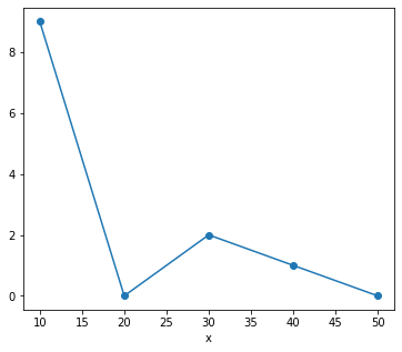
Xarray has built-in plotting, like Pandas.
da.plot(marker='o')
[<matplotlib.lines.Line2D at 0x7f6aa368eee0>]
Multidimensional DataArray
If we are just dealing with 1D data, Pandas and Xarray have very similar capabilities. Xarray’s real potential comes with multidimensional data.
Let’s analyse a multidimensional ARGO data (argo_float_4901412.npz) from ocean profiling floats.
We reload this data and examine its keys.
argo_data = np.load('argo_float_4901412.npz')
list(argo_data.keys())
['S', 'T', 'levels', 'lon', 'date', 'P', 'lat']
The values of the argo_data object are numpy arrays.
S = argo_data.f.S
T = argo_data.f.T
P = argo_data.f.P
levels = argo_data.f.levels
lon = argo_data.f.lon
lat = argo_data.f.lat
date = argo_data.f.date
print(S.shape, lon.shape, date.shape, levels.shape)
(78, 75) (75,) (75,) (78,)
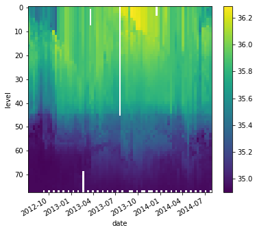
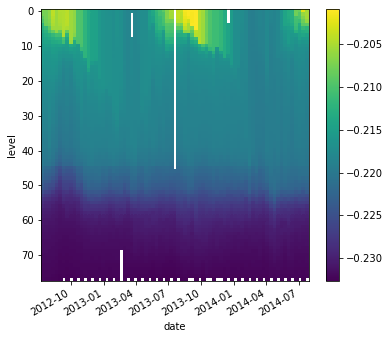
Let’s organize the data and coordinates of the salinity variable into a DataArray.
da_salinity = xr.DataArray(S, dims=['level', 'date'],
                           coords={'level': levels,
                                   'date': date},)
da_salinity
<xarray.DataArray (level: 78, date: 75)>
array([[35.6389389 , 35.51495743, 35.57297134, ..., 35.82093811,
        35.77793884, 35.66891098],
       [35.63393784, 35.5219574 , 35.57397079, ..., 35.81093216,
        35.58389664, 35.66791153],
       [35.6819458 , 35.52595901, 35.57297134, ..., 35.79592896,
        35.66290665, 35.66591263],
       ...,
       [34.91585922, 34.92390442, 34.92390442, ..., 34.93481064,
        34.94081116, 34.94680786],
       [34.91585922, 34.92390442, 34.92190552, ..., 34.93280792,
        34.93680954, 34.94380951],
       [34.91785812, 34.92390442, 34.92390442, ...,         nan,
        34.93680954,         nan]])
Coordinates:
  * level    (level) int64 0 1 2 3 4 5 6 7 8 9 ... 68 69 70 71 72 73 74 75 76 77
* date (date) datetime64[ns] 2012-07-13T22:33:06.019200 ... 2014-07-24T...- level: 78
- date: 75
- 35.64 35.51 35.57 35.4 35.45 35.5 ... 34.94 nan 34.94 nan 34.94 nan
array([[35.6389389 , 35.51495743, 35.57297134, ..., 35.82093811, 35.77793884, 35.66891098], [35.63393784, 35.5219574 , 35.57397079, ..., 35.81093216, 35.58389664, 35.66791153], [35.6819458 , 35.52595901, 35.57297134, ..., 35.79592896, 35.66290665, 35.66591263], ..., [34.91585922, 34.92390442, 34.92390442, ..., 34.93481064, 34.94081116, 34.94680786], [34.91585922, 34.92390442, 34.92190552, ..., 34.93280792, 34.93680954, 34.94380951], [34.91785812, 34.92390442, 34.92390442, ..., nan, 34.93680954, nan]]) - level(level)int640 1 2 3 4 5 6 ... 72 73 74 75 76 77
array([ 0, 1, 2, 3, 4, 5, 6, 7, 8, 9, 10, 11, 12, 13, 14, 15, 16, 17, 18, 19, 20, 21, 22, 23, 24, 25, 26, 27, 28, 29, 30, 31, 32, 33, 34, 35, 36, 37, 38, 39, 40, 41, 42, 43, 44, 45, 46, 47, 48, 49, 50, 51, 52, 53, 54, 55, 56, 57, 58, 59, 60, 61, 62, 63, 64, 65, 66, 67, 68, 69, 70, 71, 72, 73, 74, 75, 76, 77]) - date(date)datetime64[ns]2012-07-13T22:33:06.019200 ... 2...
array(['2012-07-13T22:33:06.019200000', '2012-07-23T22:54:59.990400000',
       '2012-08-02T22:55:52.003200000', '2012-08-12T23:08:59.971200000',
       '2012-08-22T23:29:01.968000000', '2012-09-01T23:17:38.976000000',
       '2012-09-12T02:59:18.960000000', '2012-09-21T23:18:37.036800000',
       '2012-10-02T03:00:17.971200000', '2012-10-11T23:13:27.984000000',
       '2012-10-22T02:50:32.006400000', '2012-10-31T23:36:39.974400000',
       '2012-11-11T02:40:46.041600000', '2012-11-20T23:08:29.990400000',
       '2012-12-01T02:47:51.993600000', '2012-12-10T23:23:16.972800000',
       '2012-12-21T02:58:48.979200000', '2012-12-30T23:07:23.030400000',
       '2013-01-10T02:56:43.008000000', '2013-01-19T23:24:26.956800000',
       '2013-01-30T02:43:53.011200000', '2013-02-08T23:15:27.043200000',
       '2013-02-19T01:12:50.976000000', '2013-02-28T23:07:13.008000000',
       '2013-03-11T02:43:30.979200000', '2013-03-20T23:17:22.992000000',
       '2013-03-31T01:50:38.025600000', '2013-04-09T23:19:07.968000000',
       '2013-04-20T02:53:29.990400000', '2013-04-29T23:28:33.024000000',
       '2013-05-10T02:50:18.009600000', '2013-05-19T23:21:05.990400000',
       '2013-05-30T02:50:30.969600000', '2013-06-08T23:32:49.027200000',
       '2013-06-19T03:42:51.004800000', '2013-06-28T23:32:16.022400000',
       '2013-07-09T03:28:30.979199999', '2013-07-18T23:33:57.974400000',
       '2013-07-29T03:15:42.019200000', '2013-08-07T23:25:02.035200000',
       '2013-08-18T01:47:44.966400000', '2013-08-28T03:02:59.020800000',
       '2013-09-07T03:03:51.984000000', '2013-09-16T23:32:07.987200000',
       '2013-09-27T04:08:27.974400000', '2013-10-06T23:25:39.964800000',
       '2013-10-17T02:55:50.995200000', '2013-10-27T03:45:47.001600000',
       '2013-11-06T01:14:52.022400000', '2013-11-16T03:29:54.009600000',
       '2013-11-26T03:03:56.995200000', '2013-12-05T23:33:59.011200000',
       '2013-12-16T02:58:01.977600000', '2013-12-25T23:22:43.017600000',
       '2014-01-05T02:52:06.009600000', '2014-01-14T23:41:18.009600000',
       '2014-01-25T03:00:43.977600000', '2014-02-03T23:29:13.977600000',
       '2014-02-14T02:50:11.961600000', '2014-02-23T23:03:21.974400000',
       '2014-03-06T02:58:03.964800000', '2014-03-15T23:10:28.012800000',
       '2014-03-26T02:51:22.032000000', '2014-04-04T23:25:58.972800000',
       '2014-04-15T03:00:45.964800000', '2014-04-24T23:24:40.003200000',
       '2014-05-05T02:56:22.012800000', '2014-05-15T00:10:06.009600000',
       '2014-05-25T03:02:43.036800000', '2014-06-03T23:34:53.961600000',
       '2014-06-14T03:01:23.980800000', '2014-06-23T23:24:31.968000000',
       '2014-07-04T03:08:30.019200000', '2014-07-13T23:47:43.008000000',
       '2014-07-24T03:02:33.014400000'], dtype='datetime64[ns]')
da_salinity.plot(yincrease=False)
<matplotlib.collections.QuadMesh at 0x7f6a9b54dbe0>
Attributes can be used to store metadata. What metadata should you store? The CF Conventions are a great resource for thinking about climate metadata. Below we define two of the required CF-conventions attributes.
da_salinity.attrs['units'] = 'PSU'
da_salinity.attrs['standard_name'] = 'sea_water_salinity'
da_salinity
<xarray.DataArray (level: 78, date: 75)>
array([[35.6389389 , 35.51495743, 35.57297134, ..., 35.82093811,
        35.77793884, 35.66891098],
       [35.63393784, 35.5219574 , 35.57397079, ..., 35.81093216,
        35.58389664, 35.66791153],
       [35.6819458 , 35.52595901, 35.57297134, ..., 35.79592896,
        35.66290665, 35.66591263],
       ...,
       [34.91585922, 34.92390442, 34.92390442, ..., 34.93481064,
        34.94081116, 34.94680786],
       [34.91585922, 34.92390442, 34.92190552, ..., 34.93280792,
        34.93680954, 34.94380951],
       [34.91785812, 34.92390442, 34.92390442, ...,         nan,
        34.93680954,         nan]])
Coordinates:
  * level    (level) int64 0 1 2 3 4 5 6 7 8 9 ... 68 69 70 71 72 73 74 75 76 77
  * date     (date) datetime64[ns] 2012-07-13T22:33:06.019200 ... 2014-07-24T...
Attributes:
    units:          PSU
standard_name: sea_water_salinity- level: 78
- date: 75
- 35.64 35.51 35.57 35.4 35.45 35.5 ... 34.94 nan 34.94 nan 34.94 nan
array([[35.6389389 , 35.51495743, 35.57297134, ..., 35.82093811, 35.77793884, 35.66891098], [35.63393784, 35.5219574 , 35.57397079, ..., 35.81093216, 35.58389664, 35.66791153], [35.6819458 , 35.52595901, 35.57297134, ..., 35.79592896, 35.66290665, 35.66591263], ..., [34.91585922, 34.92390442, 34.92390442, ..., 34.93481064, 34.94081116, 34.94680786], [34.91585922, 34.92390442, 34.92190552, ..., 34.93280792, 34.93680954, 34.94380951], [34.91785812, 34.92390442, 34.92390442, ..., nan, 34.93680954, nan]]) - level(level)int640 1 2 3 4 5 6 ... 72 73 74 75 76 77
array([ 0, 1, 2, 3, 4, 5, 6, 7, 8, 9, 10, 11, 12, 13, 14, 15, 16, 17, 18, 19, 20, 21, 22, 23, 24, 25, 26, 27, 28, 29, 30, 31, 32, 33, 34, 35, 36, 37, 38, 39, 40, 41, 42, 43, 44, 45, 46, 47, 48, 49, 50, 51, 52, 53, 54, 55, 56, 57, 58, 59, 60, 61, 62, 63, 64, 65, 66, 67, 68, 69, 70, 71, 72, 73, 74, 75, 76, 77]) - date(date)datetime64[ns]2012-07-13T22:33:06.019200 ... 2...
array(['2012-07-13T22:33:06.019200000', '2012-07-23T22:54:59.990400000',
       '2012-08-02T22:55:52.003200000', '2012-08-12T23:08:59.971200000',
       '2012-08-22T23:29:01.968000000', '2012-09-01T23:17:38.976000000',
       '2012-09-12T02:59:18.960000000', '2012-09-21T23:18:37.036800000',
       '2012-10-02T03:00:17.971200000', '2012-10-11T23:13:27.984000000',
       '2012-10-22T02:50:32.006400000', '2012-10-31T23:36:39.974400000',
       '2012-11-11T02:40:46.041600000', '2012-11-20T23:08:29.990400000',
       '2012-12-01T02:47:51.993600000', '2012-12-10T23:23:16.972800000',
       '2012-12-21T02:58:48.979200000', '2012-12-30T23:07:23.030400000',
       '2013-01-10T02:56:43.008000000', '2013-01-19T23:24:26.956800000',
       '2013-01-30T02:43:53.011200000', '2013-02-08T23:15:27.043200000',
       '2013-02-19T01:12:50.976000000', '2013-02-28T23:07:13.008000000',
       '2013-03-11T02:43:30.979200000', '2013-03-20T23:17:22.992000000',
       '2013-03-31T01:50:38.025600000', '2013-04-09T23:19:07.968000000',
       '2013-04-20T02:53:29.990400000', '2013-04-29T23:28:33.024000000',
       '2013-05-10T02:50:18.009600000', '2013-05-19T23:21:05.990400000',
       '2013-05-30T02:50:30.969600000', '2013-06-08T23:32:49.027200000',
       '2013-06-19T03:42:51.004800000', '2013-06-28T23:32:16.022400000',
       '2013-07-09T03:28:30.979199999', '2013-07-18T23:33:57.974400000',
       '2013-07-29T03:15:42.019200000', '2013-08-07T23:25:02.035200000',
       '2013-08-18T01:47:44.966400000', '2013-08-28T03:02:59.020800000',
       '2013-09-07T03:03:51.984000000', '2013-09-16T23:32:07.987200000',
       '2013-09-27T04:08:27.974400000', '2013-10-06T23:25:39.964800000',
       '2013-10-17T02:55:50.995200000', '2013-10-27T03:45:47.001600000',
       '2013-11-06T01:14:52.022400000', '2013-11-16T03:29:54.009600000',
       '2013-11-26T03:03:56.995200000', '2013-12-05T23:33:59.011200000',
       '2013-12-16T02:58:01.977600000', '2013-12-25T23:22:43.017600000',
       '2014-01-05T02:52:06.009600000', '2014-01-14T23:41:18.009600000',
       '2014-01-25T03:00:43.977600000', '2014-02-03T23:29:13.977600000',
       '2014-02-14T02:50:11.961600000', '2014-02-23T23:03:21.974400000',
       '2014-03-06T02:58:03.964800000', '2014-03-15T23:10:28.012800000',
       '2014-03-26T02:51:22.032000000', '2014-04-04T23:25:58.972800000',
       '2014-04-15T03:00:45.964800000', '2014-04-24T23:24:40.003200000',
       '2014-05-05T02:56:22.012800000', '2014-05-15T00:10:06.009600000',
       '2014-05-25T03:02:43.036800000', '2014-06-03T23:34:53.961600000',
       '2014-06-14T03:01:23.980800000', '2014-06-23T23:24:31.968000000',
       '2014-07-04T03:08:30.019200000', '2014-07-13T23:47:43.008000000',
       '2014-07-24T03:02:33.014400000'], dtype='datetime64[ns]')
- units :
- PSU
- standard_name :
- sea_water_salinity
Datasets
A Dataset holds many DataArrays which potentially can share coordinates. In analogy to pandas:
pandas.Series : pandas.Dataframe :: xarray.DataArray : xarray.Dataset
Constructing Datasets manually is a bit more involved in terms of syntax. The Dataset constructor takes three arguments:
data_varsshould be a dictionary with each key as the name of the variable and each value as one of:A
DataArrayor VariableA tuple of the form
(dims, data[, attrs]), which is converted into arguments for VariableA pandas object, which is converted into a
DataArrayA 1D array or list, which is interpreted as values for a one dimensional coordinate variable along the same dimension as it’s name
coordsshould be a dictionary of the same form as data_vars.attrsshould be a dictionary.
Let’s put together a Dataset with temperature, salinity and pressure all together
argo = xr.Dataset(
        data_vars={'salinity':    (('level', 'date'), S),
                   'temperature': (('level', 'date'), T),
                   'pressure':    (('level', 'date'), P)},
        coords={'level': levels,
                'date': date})
argo
<xarray.Dataset>
Dimensions:      (date: 75, level: 78)
Coordinates:
  * level        (level) int64 0 1 2 3 4 5 6 7 8 ... 69 70 71 72 73 74 75 76 77
  * date         (date) datetime64[ns] 2012-07-13T22:33:06.019200 ... 2014-07...
Data variables:
    salinity     (level, date) float64 35.64 35.51 35.57 35.4 ... nan 34.94 nan
    temperature  (level, date) float64 18.97 18.44 19.1 19.79 ... nan 3.714 nan
pressure (level, date) float64 6.8 6.1 6.5 5.0 ... 2e+03 nan 2e+03 nan- date: 75
- level: 78
- level(level)int640 1 2 3 4 5 6 ... 72 73 74 75 76 77
array([ 0, 1, 2, 3, 4, 5, 6, 7, 8, 9, 10, 11, 12, 13, 14, 15, 16, 17, 18, 19, 20, 21, 22, 23, 24, 25, 26, 27, 28, 29, 30, 31, 32, 33, 34, 35, 36, 37, 38, 39, 40, 41, 42, 43, 44, 45, 46, 47, 48, 49, 50, 51, 52, 53, 54, 55, 56, 57, 58, 59, 60, 61, 62, 63, 64, 65, 66, 67, 68, 69, 70, 71, 72, 73, 74, 75, 76, 77]) - date(date)datetime64[ns]2012-07-13T22:33:06.019200 ... 2...
array(['2012-07-13T22:33:06.019200000', '2012-07-23T22:54:59.990400000',
       '2012-08-02T22:55:52.003200000', '2012-08-12T23:08:59.971200000',
       '2012-08-22T23:29:01.968000000', '2012-09-01T23:17:38.976000000',
       '2012-09-12T02:59:18.960000000', '2012-09-21T23:18:37.036800000',
       '2012-10-02T03:00:17.971200000', '2012-10-11T23:13:27.984000000',
       '2012-10-22T02:50:32.006400000', '2012-10-31T23:36:39.974400000',
       '2012-11-11T02:40:46.041600000', '2012-11-20T23:08:29.990400000',
       '2012-12-01T02:47:51.993600000', '2012-12-10T23:23:16.972800000',
       '2012-12-21T02:58:48.979200000', '2012-12-30T23:07:23.030400000',
       '2013-01-10T02:56:43.008000000', '2013-01-19T23:24:26.956800000',
       '2013-01-30T02:43:53.011200000', '2013-02-08T23:15:27.043200000',
       '2013-02-19T01:12:50.976000000', '2013-02-28T23:07:13.008000000',
       '2013-03-11T02:43:30.979200000', '2013-03-20T23:17:22.992000000',
       '2013-03-31T01:50:38.025600000', '2013-04-09T23:19:07.968000000',
       '2013-04-20T02:53:29.990400000', '2013-04-29T23:28:33.024000000',
       '2013-05-10T02:50:18.009600000', '2013-05-19T23:21:05.990400000',
       '2013-05-30T02:50:30.969600000', '2013-06-08T23:32:49.027200000',
       '2013-06-19T03:42:51.004800000', '2013-06-28T23:32:16.022400000',
       '2013-07-09T03:28:30.979199999', '2013-07-18T23:33:57.974400000',
       '2013-07-29T03:15:42.019200000', '2013-08-07T23:25:02.035200000',
       '2013-08-18T01:47:44.966400000', '2013-08-28T03:02:59.020800000',
       '2013-09-07T03:03:51.984000000', '2013-09-16T23:32:07.987200000',
       '2013-09-27T04:08:27.974400000', '2013-10-06T23:25:39.964800000',
       '2013-10-17T02:55:50.995200000', '2013-10-27T03:45:47.001600000',
       '2013-11-06T01:14:52.022400000', '2013-11-16T03:29:54.009600000',
       '2013-11-26T03:03:56.995200000', '2013-12-05T23:33:59.011200000',
       '2013-12-16T02:58:01.977600000', '2013-12-25T23:22:43.017600000',
       '2014-01-05T02:52:06.009600000', '2014-01-14T23:41:18.009600000',
       '2014-01-25T03:00:43.977600000', '2014-02-03T23:29:13.977600000',
       '2014-02-14T02:50:11.961600000', '2014-02-23T23:03:21.974400000',
       '2014-03-06T02:58:03.964800000', '2014-03-15T23:10:28.012800000',
       '2014-03-26T02:51:22.032000000', '2014-04-04T23:25:58.972800000',
       '2014-04-15T03:00:45.964800000', '2014-04-24T23:24:40.003200000',
       '2014-05-05T02:56:22.012800000', '2014-05-15T00:10:06.009600000',
       '2014-05-25T03:02:43.036800000', '2014-06-03T23:34:53.961600000',
       '2014-06-14T03:01:23.980800000', '2014-06-23T23:24:31.968000000',
       '2014-07-04T03:08:30.019200000', '2014-07-13T23:47:43.008000000',
       '2014-07-24T03:02:33.014400000'], dtype='datetime64[ns]')
- salinity(level, date)float6435.64 35.51 35.57 ... nan 34.94 nan
array([[35.6389389 , 35.51495743, 35.57297134, ..., 35.82093811, 35.77793884, 35.66891098], [35.63393784, 35.5219574 , 35.57397079, ..., 35.81093216, 35.58389664, 35.66791153], [35.6819458 , 35.52595901, 35.57297134, ..., 35.79592896, 35.66290665, 35.66591263], ..., [34.91585922, 34.92390442, 34.92390442, ..., 34.93481064, 34.94081116, 34.94680786], [34.91585922, 34.92390442, 34.92190552, ..., 34.93280792, 34.93680954, 34.94380951], [34.91785812, 34.92390442, 34.92390442, ..., nan, 34.93680954, nan]]) - temperature(level, date)float6418.97 18.44 19.1 ... nan 3.714 nan
array([[18.97400093, 18.43700027, 19.09900093, ..., 19.11300087, 21.82299995, 20.13100052], [18.74099922, 18.39999962, 19.08200073, ..., 18.47200012, 19.45999908, 20.125 ], [18.37000084, 18.37400055, 19.06500053, ..., 18.22999954, 19.26199913, 20.07699966], ..., [ 3.79299998, 3.81399989, 3.80200005, ..., 3.80699992, 3.81100011, 3.8599999 ], [ 3.76399994, 3.77800012, 3.75699997, ..., 3.75399995, 3.74600005, 3.80599999], [ 3.74399996, 3.74600005, 3.7249999 , ..., nan, 3.71399999, nan]]) - pressure(level, date)float646.8 6.1 6.5 5.0 ... nan 2e+03 nan
array([[   6.80000019,    6.0999999 ,    6.5       , ...,    7.0999999 ,
           7.20000029,    6.5       ],
       [  10.69999981,   10.59999943,   10.39999962, ...,   10.79999924,
          11.09999943,   10.39999962],
       [  15.69999981,   14.09999943,   14.89999962, ...,   15.89999962,
          15.59999943,   15.89999962],
       ...,
       [1900.60009766, 1900.        , 1900.19995117, ..., 1899.70007324,
        1900.40002441, 1899.80004883],
       [1949.90002441, 1950.        , 1949.89990234, ..., 1950.59997559,
        1950.20007324, 1949.70007324],
       [1999.30004883, 1998.        , 1998.5       , ...,           nan,
        2000.40002441,           nan]])
What about lon and lat? We forgot them in the creation process, but we can add them after
argo.coords['lon'] = lon
argo
<xarray.Dataset>
Dimensions:      (date: 75, level: 78, lon: 75)
Coordinates:
  * level        (level) int64 0 1 2 3 4 5 6 7 8 ... 69 70 71 72 73 74 75 76 77
  * date         (date) datetime64[ns] 2012-07-13T22:33:06.019200 ... 2014-07...
  * lon          (lon) float64 -39.13 -37.28 -36.9 ... -33.83 -34.11 -34.38
Data variables:
    salinity     (level, date) float64 35.64 35.51 35.57 35.4 ... nan 34.94 nan
    temperature  (level, date) float64 18.97 18.44 19.1 19.79 ... nan 3.714 nan
pressure (level, date) float64 6.8 6.1 6.5 5.0 ... 2e+03 nan 2e+03 nan- date: 75
- level: 78
- lon: 75
- level(level)int640 1 2 3 4 5 6 ... 72 73 74 75 76 77
array([ 0, 1, 2, 3, 4, 5, 6, 7, 8, 9, 10, 11, 12, 13, 14, 15, 16, 17, 18, 19, 20, 21, 22, 23, 24, 25, 26, 27, 28, 29, 30, 31, 32, 33, 34, 35, 36, 37, 38, 39, 40, 41, 42, 43, 44, 45, 46, 47, 48, 49, 50, 51, 52, 53, 54, 55, 56, 57, 58, 59, 60, 61, 62, 63, 64, 65, 66, 67, 68, 69, 70, 71, 72, 73, 74, 75, 76, 77]) - date(date)datetime64[ns]2012-07-13T22:33:06.019200 ... 2...
array(['2012-07-13T22:33:06.019200000', '2012-07-23T22:54:59.990400000', '2012-08-02T22:55:52.003200000', '2012-08-12T23:08:59.971200000', '2012-08-22T23:29:01.968000000', '2012-09-01T23:17:38.976000000', '2012-09-12T02:59:18.960000000', '2012-09-21T23:18:37.036800000', '2012-10-02T03:00:17.971200000', '2012-10-11T23:13:27.984000000', '2012-10-22T02:50:32.006400000', '2012-10-31T23:36:39.974400000', '2012-11-11T02:40:46.041600000', '2012-11-20T23:08:29.990400000', '2012-12-01T02:47:51.993600000', '2012-12-10T23:23:16.972800000', '2012-12-21T02:58:48.979200000', '2012-12-30T23:07:23.030400000', '2013-01-10T02:56:43.008000000', '2013-01-19T23:24:26.956800000', '2013-01-30T02:43:53.011200000', '2013-02-08T23:15:27.043200000', '2013-02-19T01:12:50.976000000', '2013-02-28T23:07:13.008000000', '2013-03-11T02:43:30.979200000', '2013-03-20T23:17:22.992000000', '2013-03-31T01:50:38.025600000', '2013-04-09T23:19:07.968000000', '2013-04-20T02:53:29.990400000', '2013-04-29T23:28:33.024000000', '2013-05-10T02:50:18.009600000', '2013-05-19T23:21:05.990400000', '2013-05-30T02:50:30.969600000', '2013-06-08T23:32:49.027200000', '2013-06-19T03:42:51.004800000', '2013-06-28T23:32:16.022400000', '2013-07-09T03:28:30.979199999', '2013-07-18T23:33:57.974400000', '2013-07-29T03:15:42.019200000', '2013-08-07T23:25:02.035200000', '2013-08-18T01:47:44.966400000', '2013-08-28T03:02:59.020800000', '2013-09-07T03:03:51.984000000', '2013-09-16T23:32:07.987200000', '2013-09-27T04:08:27.974400000', '2013-10-06T23:25:39.964800000', '2013-10-17T02:55:50.995200000', '2013-10-27T03:45:47.001600000', '2013-11-06T01:14:52.022400000', '2013-11-16T03:29:54.009600000', '2013-11-26T03:03:56.995200000', '2013-12-05T23:33:59.011200000', '2013-12-16T02:58:01.977600000', '2013-12-25T23:22:43.017600000', '2014-01-05T02:52:06.009600000', '2014-01-14T23:41:18.009600000', '2014-01-25T03:00:43.977600000', '2014-02-03T23:29:13.977600000', '2014-02-14T02:50:11.961600000', '2014-02-23T23:03:21.974400000', '2014-03-06T02:58:03.964800000', '2014-03-15T23:10:28.012800000', '2014-03-26T02:51:22.032000000', '2014-04-04T23:25:58.972800000', '2014-04-15T03:00:45.964800000', '2014-04-24T23:24:40.003200000', '2014-05-05T02:56:22.012800000', '2014-05-15T00:10:06.009600000', '2014-05-25T03:02:43.036800000', '2014-06-03T23:34:53.961600000', '2014-06-14T03:01:23.980800000', '2014-06-23T23:24:31.968000000', '2014-07-04T03:08:30.019200000', '2014-07-13T23:47:43.008000000', '2014-07-24T03:02:33.014400000'], dtype='datetime64[ns]') - lon(lon)float64-39.13 -37.28 ... -34.11 -34.38
array([-39.13 , -37.282, -36.9  , -36.89 , -37.053, -36.658, -35.963, -35.184,
       -34.462, -33.784, -32.972, -32.546, -32.428, -32.292, -32.169, -31.998,
       -31.824, -31.624, -31.433, -31.312, -31.107, -31.147, -31.044, -31.14 ,
       -31.417, -31.882, -32.145, -32.487, -32.537, -32.334, -32.042, -31.892,
       -31.861, -31.991, -31.883, -31.89 , -31.941, -31.889, -31.724, -31.412,
       -31.786, -31.561, -31.732, -31.553, -31.862, -32.389, -32.318, -32.19 ,
       -32.224, -32.368, -32.306, -32.305, -32.65 , -33.093, -33.263, -33.199,
       -33.27 , -33.237, -33.221, -33.011, -32.844, -32.981, -32.784, -32.607,
       -32.87 , -33.196, -33.524, -33.956, -33.944, -33.71 , -33.621, -33.552,
       -33.828, -34.11 , -34.38 ])
- salinity(level, date)float6435.64 35.51 35.57 ... nan 34.94 nan
array([[35.6389389 , 35.51495743, 35.57297134, ..., 35.82093811, 35.77793884, 35.66891098], [35.63393784, 35.5219574 , 35.57397079, ..., 35.81093216, 35.58389664, 35.66791153], [35.6819458 , 35.52595901, 35.57297134, ..., 35.79592896, 35.66290665, 35.66591263], ..., [34.91585922, 34.92390442, 34.92390442, ..., 34.93481064, 34.94081116, 34.94680786], [34.91585922, 34.92390442, 34.92190552, ..., 34.93280792, 34.93680954, 34.94380951], [34.91785812, 34.92390442, 34.92390442, ..., nan, 34.93680954, nan]]) - temperature(level, date)float6418.97 18.44 19.1 ... nan 3.714 nan
array([[18.97400093, 18.43700027, 19.09900093, ..., 19.11300087, 21.82299995, 20.13100052], [18.74099922, 18.39999962, 19.08200073, ..., 18.47200012, 19.45999908, 20.125 ], [18.37000084, 18.37400055, 19.06500053, ..., 18.22999954, 19.26199913, 20.07699966], ..., [ 3.79299998, 3.81399989, 3.80200005, ..., 3.80699992, 3.81100011, 3.8599999 ], [ 3.76399994, 3.77800012, 3.75699997, ..., 3.75399995, 3.74600005, 3.80599999], [ 3.74399996, 3.74600005, 3.7249999 , ..., nan, 3.71399999, nan]]) - pressure(level, date)float646.8 6.1 6.5 5.0 ... nan 2e+03 nan
array([[   6.80000019,    6.0999999 ,    6.5       , ...,    7.0999999 ,
           7.20000029,    6.5       ],
       [  10.69999981,   10.59999943,   10.39999962, ...,   10.79999924,
          11.09999943,   10.39999962],
       [  15.69999981,   14.09999943,   14.89999962, ...,   15.89999962,
          15.59999943,   15.89999962],
       ...,
       [1900.60009766, 1900.        , 1900.19995117, ..., 1899.70007324,
        1900.40002441, 1899.80004883],
       [1949.90002441, 1950.        , 1949.89990234, ..., 1950.59997559,
        1950.20007324, 1949.70007324],
       [1999.30004883, 1998.        , 1998.5       , ...,           nan,
        2000.40002441,           nan]])
That was not quite right…we want lon to have dimension date:
del argo['lon']
argo.coords['lon'] = ('date', lon)
argo.coords['lat'] = ('date', lat)
argo
<xarray.Dataset>
Dimensions:      (date: 75, level: 78)
Coordinates:
  * level        (level) int64 0 1 2 3 4 5 6 7 8 ... 69 70 71 72 73 74 75 76 77
  * date         (date) datetime64[ns] 2012-07-13T22:33:06.019200 ... 2014-07...
    lon          (date) float64 -39.13 -37.28 -36.9 ... -33.83 -34.11 -34.38
    lat          (date) float64 47.19 46.72 46.45 46.23 ... 42.6 42.46 42.38
Data variables:
    salinity     (level, date) float64 35.64 35.51 35.57 35.4 ... nan 34.94 nan
    temperature  (level, date) float64 18.97 18.44 19.1 19.79 ... nan 3.714 nan
pressure (level, date) float64 6.8 6.1 6.5 5.0 ... 2e+03 nan 2e+03 nan- date: 75
- level: 78
- level(level)int640 1 2 3 4 5 6 ... 72 73 74 75 76 77
array([ 0, 1, 2, 3, 4, 5, 6, 7, 8, 9, 10, 11, 12, 13, 14, 15, 16, 17, 18, 19, 20, 21, 22, 23, 24, 25, 26, 27, 28, 29, 30, 31, 32, 33, 34, 35, 36, 37, 38, 39, 40, 41, 42, 43, 44, 45, 46, 47, 48, 49, 50, 51, 52, 53, 54, 55, 56, 57, 58, 59, 60, 61, 62, 63, 64, 65, 66, 67, 68, 69, 70, 71, 72, 73, 74, 75, 76, 77]) - date(date)datetime64[ns]2012-07-13T22:33:06.019200 ... 2...
array(['2012-07-13T22:33:06.019200000', '2012-07-23T22:54:59.990400000', '2012-08-02T22:55:52.003200000', '2012-08-12T23:08:59.971200000', '2012-08-22T23:29:01.968000000', '2012-09-01T23:17:38.976000000', '2012-09-12T02:59:18.960000000', '2012-09-21T23:18:37.036800000', '2012-10-02T03:00:17.971200000', '2012-10-11T23:13:27.984000000', '2012-10-22T02:50:32.006400000', '2012-10-31T23:36:39.974400000', '2012-11-11T02:40:46.041600000', '2012-11-20T23:08:29.990400000', '2012-12-01T02:47:51.993600000', '2012-12-10T23:23:16.972800000', '2012-12-21T02:58:48.979200000', '2012-12-30T23:07:23.030400000', '2013-01-10T02:56:43.008000000', '2013-01-19T23:24:26.956800000', '2013-01-30T02:43:53.011200000', '2013-02-08T23:15:27.043200000', '2013-02-19T01:12:50.976000000', '2013-02-28T23:07:13.008000000', '2013-03-11T02:43:30.979200000', '2013-03-20T23:17:22.992000000', '2013-03-31T01:50:38.025600000', '2013-04-09T23:19:07.968000000', '2013-04-20T02:53:29.990400000', '2013-04-29T23:28:33.024000000', '2013-05-10T02:50:18.009600000', '2013-05-19T23:21:05.990400000', '2013-05-30T02:50:30.969600000', '2013-06-08T23:32:49.027200000', '2013-06-19T03:42:51.004800000', '2013-06-28T23:32:16.022400000', '2013-07-09T03:28:30.979199999', '2013-07-18T23:33:57.974400000', '2013-07-29T03:15:42.019200000', '2013-08-07T23:25:02.035200000', '2013-08-18T01:47:44.966400000', '2013-08-28T03:02:59.020800000', '2013-09-07T03:03:51.984000000', '2013-09-16T23:32:07.987200000', '2013-09-27T04:08:27.974400000', '2013-10-06T23:25:39.964800000', '2013-10-17T02:55:50.995200000', '2013-10-27T03:45:47.001600000', '2013-11-06T01:14:52.022400000', '2013-11-16T03:29:54.009600000', '2013-11-26T03:03:56.995200000', '2013-12-05T23:33:59.011200000', '2013-12-16T02:58:01.977600000', '2013-12-25T23:22:43.017600000', '2014-01-05T02:52:06.009600000', '2014-01-14T23:41:18.009600000', '2014-01-25T03:00:43.977600000', '2014-02-03T23:29:13.977600000', '2014-02-14T02:50:11.961600000', '2014-02-23T23:03:21.974400000', '2014-03-06T02:58:03.964800000', '2014-03-15T23:10:28.012800000', '2014-03-26T02:51:22.032000000', '2014-04-04T23:25:58.972800000', '2014-04-15T03:00:45.964800000', '2014-04-24T23:24:40.003200000', '2014-05-05T02:56:22.012800000', '2014-05-15T00:10:06.009600000', '2014-05-25T03:02:43.036800000', '2014-06-03T23:34:53.961600000', '2014-06-14T03:01:23.980800000', '2014-06-23T23:24:31.968000000', '2014-07-04T03:08:30.019200000', '2014-07-13T23:47:43.008000000', '2014-07-24T03:02:33.014400000'], dtype='datetime64[ns]') - lon(date)float64-39.13 -37.28 ... -34.11 -34.38
array([-39.13 , -37.282, -36.9 , -36.89 , -37.053, -36.658, -35.963, -35.184, -34.462, -33.784, -32.972, -32.546, -32.428, -32.292, -32.169, -31.998, -31.824, -31.624, -31.433, -31.312, -31.107, -31.147, -31.044, -31.14 , -31.417, -31.882, -32.145, -32.487, -32.537, -32.334, -32.042, -31.892, -31.861, -31.991, -31.883, -31.89 , -31.941, -31.889, -31.724, -31.412, -31.786, -31.561, -31.732, -31.553, -31.862, -32.389, -32.318, -32.19 , -32.224, -32.368, -32.306, -32.305, -32.65 , -33.093, -33.263, -33.199, -33.27 , -33.237, -33.221, -33.011, -32.844, -32.981, -32.784, -32.607, -32.87 , -33.196, -33.524, -33.956, -33.944, -33.71 , -33.621, -33.552, -33.828, -34.11 , -34.38 ]) - lat(date)float6447.19 46.72 46.45 ... 42.46 42.38
array([47.187, 46.716, 46.45 , 46.23 , 45.459, 44.833, 44.452, 44.839,
       44.956, 44.676, 44.13 , 43.644, 43.067, 42.662, 42.513, 42.454,
       42.396, 42.256, 42.089, 41.944, 41.712, 41.571, 41.596, 41.581,
       41.351, 41.032, 40.912, 40.792, 40.495, 40.383, 40.478, 40.672,
       41.032, 40.864, 40.651, 40.425, 40.228, 40.197, 40.483, 40.311,
       40.457, 40.463, 40.164, 40.047, 39.963, 40.122, 40.57 , 40.476,
       40.527, 40.589, 40.749, 40.993, 41.162, 41.237, 41.448, 41.65 ,
       42.053, 42.311, 42.096, 41.683, 41.661, 41.676, 42.018, 42.395,
       42.532, 42.558, 42.504, 42.63 , 42.934, 42.952, 42.777, 42.722,
       42.601, 42.457, 42.379])
- salinity(level, date)float6435.64 35.51 35.57 ... nan 34.94 nan
array([[35.6389389 , 35.51495743, 35.57297134, ..., 35.82093811, 35.77793884, 35.66891098], [35.63393784, 35.5219574 , 35.57397079, ..., 35.81093216, 35.58389664, 35.66791153], [35.6819458 , 35.52595901, 35.57297134, ..., 35.79592896, 35.66290665, 35.66591263], ..., [34.91585922, 34.92390442, 34.92390442, ..., 34.93481064, 34.94081116, 34.94680786], [34.91585922, 34.92390442, 34.92190552, ..., 34.93280792, 34.93680954, 34.94380951], [34.91785812, 34.92390442, 34.92390442, ..., nan, 34.93680954, nan]]) - temperature(level, date)float6418.97 18.44 19.1 ... nan 3.714 nan
array([[18.97400093, 18.43700027, 19.09900093, ..., 19.11300087, 21.82299995, 20.13100052], [18.74099922, 18.39999962, 19.08200073, ..., 18.47200012, 19.45999908, 20.125 ], [18.37000084, 18.37400055, 19.06500053, ..., 18.22999954, 19.26199913, 20.07699966], ..., [ 3.79299998, 3.81399989, 3.80200005, ..., 3.80699992, 3.81100011, 3.8599999 ], [ 3.76399994, 3.77800012, 3.75699997, ..., 3.75399995, 3.74600005, 3.80599999], [ 3.74399996, 3.74600005, 3.7249999 , ..., nan, 3.71399999, nan]]) - pressure(level, date)float646.8 6.1 6.5 5.0 ... nan 2e+03 nan
array([[   6.80000019,    6.0999999 ,    6.5       , ...,    7.0999999 ,
           7.20000029,    6.5       ],
       [  10.69999981,   10.59999943,   10.39999962, ...,   10.79999924,
          11.09999943,   10.39999962],
       [  15.69999981,   14.09999943,   14.89999962, ...,   15.89999962,
          15.59999943,   15.89999962],
       ...,
       [1900.60009766, 1900.        , 1900.19995117, ..., 1899.70007324,
        1900.40002441, 1899.80004883],
       [1949.90002441, 1950.        , 1949.89990234, ..., 1950.59997559,
        1950.20007324, 1949.70007324],
       [1999.30004883, 1998.        , 1998.5       , ...,           nan,
        2000.40002441,           nan]])
Coordinates vs. Data Variables
Data variables can be modified through arithmentic operations or other functions. Coordinates are always keept the same.
argo * 10000
<xarray.Dataset>
Dimensions:      (date: 75, level: 78)
Coordinates:
  * level        (level) int64 0 1 2 3 4 5 6 7 8 ... 69 70 71 72 73 74 75 76 77
  * date         (date) datetime64[ns] 2012-07-13T22:33:06.019200 ... 2014-07...
    lon          (date) float64 -39.13 -37.28 -36.9 ... -33.83 -34.11 -34.38
    lat          (date) float64 47.19 46.72 46.45 46.23 ... 42.6 42.46 42.38
Data variables:
    salinity     (level, date) float64 3.564e+05 3.551e+05 ... 3.494e+05 nan
    temperature  (level, date) float64 1.897e+05 1.844e+05 ... 3.714e+04 nan
pressure (level, date) float64 6.8e+04 6.1e+04 6.5e+04 ... nan 2e+07 nan- date: 75
- level: 78
- level(level)int640 1 2 3 4 5 6 ... 72 73 74 75 76 77
array([ 0, 1, 2, 3, 4, 5, 6, 7, 8, 9, 10, 11, 12, 13, 14, 15, 16, 17, 18, 19, 20, 21, 22, 23, 24, 25, 26, 27, 28, 29, 30, 31, 32, 33, 34, 35, 36, 37, 38, 39, 40, 41, 42, 43, 44, 45, 46, 47, 48, 49, 50, 51, 52, 53, 54, 55, 56, 57, 58, 59, 60, 61, 62, 63, 64, 65, 66, 67, 68, 69, 70, 71, 72, 73, 74, 75, 76, 77]) - date(date)datetime64[ns]2012-07-13T22:33:06.019200 ... 2...
array(['2012-07-13T22:33:06.019200000', '2012-07-23T22:54:59.990400000', '2012-08-02T22:55:52.003200000', '2012-08-12T23:08:59.971200000', '2012-08-22T23:29:01.968000000', '2012-09-01T23:17:38.976000000', '2012-09-12T02:59:18.960000000', '2012-09-21T23:18:37.036800000', '2012-10-02T03:00:17.971200000', '2012-10-11T23:13:27.984000000', '2012-10-22T02:50:32.006400000', '2012-10-31T23:36:39.974400000', '2012-11-11T02:40:46.041600000', '2012-11-20T23:08:29.990400000', '2012-12-01T02:47:51.993600000', '2012-12-10T23:23:16.972800000', '2012-12-21T02:58:48.979200000', '2012-12-30T23:07:23.030400000', '2013-01-10T02:56:43.008000000', '2013-01-19T23:24:26.956800000', '2013-01-30T02:43:53.011200000', '2013-02-08T23:15:27.043200000', '2013-02-19T01:12:50.976000000', '2013-02-28T23:07:13.008000000', '2013-03-11T02:43:30.979200000', '2013-03-20T23:17:22.992000000', '2013-03-31T01:50:38.025600000', '2013-04-09T23:19:07.968000000', '2013-04-20T02:53:29.990400000', '2013-04-29T23:28:33.024000000', '2013-05-10T02:50:18.009600000', '2013-05-19T23:21:05.990400000', '2013-05-30T02:50:30.969600000', '2013-06-08T23:32:49.027200000', '2013-06-19T03:42:51.004800000', '2013-06-28T23:32:16.022400000', '2013-07-09T03:28:30.979199999', '2013-07-18T23:33:57.974400000', '2013-07-29T03:15:42.019200000', '2013-08-07T23:25:02.035200000', '2013-08-18T01:47:44.966400000', '2013-08-28T03:02:59.020800000', '2013-09-07T03:03:51.984000000', '2013-09-16T23:32:07.987200000', '2013-09-27T04:08:27.974400000', '2013-10-06T23:25:39.964800000', '2013-10-17T02:55:50.995200000', '2013-10-27T03:45:47.001600000', '2013-11-06T01:14:52.022400000', '2013-11-16T03:29:54.009600000', '2013-11-26T03:03:56.995200000', '2013-12-05T23:33:59.011200000', '2013-12-16T02:58:01.977600000', '2013-12-25T23:22:43.017600000', '2014-01-05T02:52:06.009600000', '2014-01-14T23:41:18.009600000', '2014-01-25T03:00:43.977600000', '2014-02-03T23:29:13.977600000', '2014-02-14T02:50:11.961600000', '2014-02-23T23:03:21.974400000', '2014-03-06T02:58:03.964800000', '2014-03-15T23:10:28.012800000', '2014-03-26T02:51:22.032000000', '2014-04-04T23:25:58.972800000', '2014-04-15T03:00:45.964800000', '2014-04-24T23:24:40.003200000', '2014-05-05T02:56:22.012800000', '2014-05-15T00:10:06.009600000', '2014-05-25T03:02:43.036800000', '2014-06-03T23:34:53.961600000', '2014-06-14T03:01:23.980800000', '2014-06-23T23:24:31.968000000', '2014-07-04T03:08:30.019200000', '2014-07-13T23:47:43.008000000', '2014-07-24T03:02:33.014400000'], dtype='datetime64[ns]') - lon(date)float64-39.13 -37.28 ... -34.11 -34.38
array([-39.13 , -37.282, -36.9 , -36.89 , -37.053, -36.658, -35.963, -35.184, -34.462, -33.784, -32.972, -32.546, -32.428, -32.292, -32.169, -31.998, -31.824, -31.624, -31.433, -31.312, -31.107, -31.147, -31.044, -31.14 , -31.417, -31.882, -32.145, -32.487, -32.537, -32.334, -32.042, -31.892, -31.861, -31.991, -31.883, -31.89 , -31.941, -31.889, -31.724, -31.412, -31.786, -31.561, -31.732, -31.553, -31.862, -32.389, -32.318, -32.19 , -32.224, -32.368, -32.306, -32.305, -32.65 , -33.093, -33.263, -33.199, -33.27 , -33.237, -33.221, -33.011, -32.844, -32.981, -32.784, -32.607, -32.87 , -33.196, -33.524, -33.956, -33.944, -33.71 , -33.621, -33.552, -33.828, -34.11 , -34.38 ]) - lat(date)float6447.19 46.72 46.45 ... 42.46 42.38
array([47.187, 46.716, 46.45 , 46.23 , 45.459, 44.833, 44.452, 44.839,
       44.956, 44.676, 44.13 , 43.644, 43.067, 42.662, 42.513, 42.454,
       42.396, 42.256, 42.089, 41.944, 41.712, 41.571, 41.596, 41.581,
       41.351, 41.032, 40.912, 40.792, 40.495, 40.383, 40.478, 40.672,
       41.032, 40.864, 40.651, 40.425, 40.228, 40.197, 40.483, 40.311,
       40.457, 40.463, 40.164, 40.047, 39.963, 40.122, 40.57 , 40.476,
       40.527, 40.589, 40.749, 40.993, 41.162, 41.237, 41.448, 41.65 ,
       42.053, 42.311, 42.096, 41.683, 41.661, 41.676, 42.018, 42.395,
       42.532, 42.558, 42.504, 42.63 , 42.934, 42.952, 42.777, 42.722,
       42.601, 42.457, 42.379])
- salinity(level, date)float643.564e+05 3.551e+05 ... nan
array([[356389.38903809, 355149.57427979, 355729.71343994, ..., 358209.38110352, 357779.38842773, 356689.10980225], [356339.37835693, 355219.57397461, 355739.70794678, ..., 358109.32159424, 355838.96636963, 356679.11529541], [356819.45800781, 355259.59014893, 355729.71343994, ..., 357959.28955078, 356629.06646729, 356659.12628174], ..., [349158.59222412, 349239.04418945, 349239.04418945, ..., 349348.10638428, 349408.11157227, 349468.07861328], [349158.59222412, 349239.04418945, 349219.05517578, ..., 349328.07922363, 349368.09539795, 349438.09509277], [349178.58123779, 349239.04418945, 349239.04418945, ..., nan, 349368.09539795, nan]]) - temperature(level, date)float641.897e+05 1.844e+05 ... nan
array([[189740.00930786, 184370.00274658, 190990.00930786, ..., 191130.00869751, 218229.99954224, 201310.00518799], [187409.99221802, 183999.9961853 , 190820.00732422, ..., 184720.0012207 , 194599.99084473, 201250. ], [183700.00839233, 183740.00549316, 190650.00534058, ..., 182299.99542236, 192619.99130249, 200769.99664307], ..., [ 37929.99982834, 38139.99891281, 38020.00045776, ..., 38069.99921799, 38110.00108719, 38599.99895096], [ 37639.99938965, 37780.00116348, 37569.99969482, ..., 37539.99948502, 37460.00051498, 38059.99994278], [ 37439.99958038, 37460.00051498, 37249.99904633, ..., nan, 37139.99986649, nan]]) - pressure(level, date)float646.8e+04 6.1e+04 ... 2e+07 nan
array([[   68000.00190735,    60999.99904633,    65000.        , ...,
           70999.99904633,    72000.00286102,    65000.        ],
       [  106999.99809265,   105999.99427795,   103999.9961853 , ...,
          107999.99237061,   110999.99427795,   103999.9961853 ],
       [  156999.99809265,   140999.99427795,   148999.9961853 , ...,
          158999.9961853 ,   155999.99427795,   158999.9961853 ],
       ...,
       [19006000.9765625 , 19000000.        , 19001999.51171875, ...,
        18997000.73242188, 19004000.24414062, 18998000.48828125],
       [19499000.24414062, 19500000.        , 19498999.0234375 , ...,
        19505999.75585938, 19502000.73242188, 19497000.73242188],
       [19993000.48828125, 19980000.        , 19985000.        , ...,
                      nan, 20004000.24414062,               nan]])
Clearly lon and lat are coordinates rather than data variables. We can change their status as follows:
argo = argo.set_coords(['lon', 'lat'])
argo
<xarray.Dataset>
Dimensions:      (date: 75, level: 78)
Coordinates:
  * level        (level) int64 0 1 2 3 4 5 6 7 8 ... 69 70 71 72 73 74 75 76 77
  * date         (date) datetime64[ns] 2012-07-13T22:33:06.019200 ... 2014-07...
    lon          (date) float64 -39.13 -37.28 -36.9 ... -33.83 -34.11 -34.38
    lat          (date) float64 47.19 46.72 46.45 46.23 ... 42.6 42.46 42.38
Data variables:
    salinity     (level, date) float64 35.64 35.51 35.57 35.4 ... nan 34.94 nan
    temperature  (level, date) float64 18.97 18.44 19.1 19.79 ... nan 3.714 nan
pressure (level, date) float64 6.8 6.1 6.5 5.0 ... 2e+03 nan 2e+03 nan- date: 75
- level: 78
- level(level)int640 1 2 3 4 5 6 ... 72 73 74 75 76 77
array([ 0, 1, 2, 3, 4, 5, 6, 7, 8, 9, 10, 11, 12, 13, 14, 15, 16, 17, 18, 19, 20, 21, 22, 23, 24, 25, 26, 27, 28, 29, 30, 31, 32, 33, 34, 35, 36, 37, 38, 39, 40, 41, 42, 43, 44, 45, 46, 47, 48, 49, 50, 51, 52, 53, 54, 55, 56, 57, 58, 59, 60, 61, 62, 63, 64, 65, 66, 67, 68, 69, 70, 71, 72, 73, 74, 75, 76, 77]) - date(date)datetime64[ns]2012-07-13T22:33:06.019200 ... 2...
array(['2012-07-13T22:33:06.019200000', '2012-07-23T22:54:59.990400000', '2012-08-02T22:55:52.003200000', '2012-08-12T23:08:59.971200000', '2012-08-22T23:29:01.968000000', '2012-09-01T23:17:38.976000000', '2012-09-12T02:59:18.960000000', '2012-09-21T23:18:37.036800000', '2012-10-02T03:00:17.971200000', '2012-10-11T23:13:27.984000000', '2012-10-22T02:50:32.006400000', '2012-10-31T23:36:39.974400000', '2012-11-11T02:40:46.041600000', '2012-11-20T23:08:29.990400000', '2012-12-01T02:47:51.993600000', '2012-12-10T23:23:16.972800000', '2012-12-21T02:58:48.979200000', '2012-12-30T23:07:23.030400000', '2013-01-10T02:56:43.008000000', '2013-01-19T23:24:26.956800000', '2013-01-30T02:43:53.011200000', '2013-02-08T23:15:27.043200000', '2013-02-19T01:12:50.976000000', '2013-02-28T23:07:13.008000000', '2013-03-11T02:43:30.979200000', '2013-03-20T23:17:22.992000000', '2013-03-31T01:50:38.025600000', '2013-04-09T23:19:07.968000000', '2013-04-20T02:53:29.990400000', '2013-04-29T23:28:33.024000000', '2013-05-10T02:50:18.009600000', '2013-05-19T23:21:05.990400000', '2013-05-30T02:50:30.969600000', '2013-06-08T23:32:49.027200000', '2013-06-19T03:42:51.004800000', '2013-06-28T23:32:16.022400000', '2013-07-09T03:28:30.979199999', '2013-07-18T23:33:57.974400000', '2013-07-29T03:15:42.019200000', '2013-08-07T23:25:02.035200000', '2013-08-18T01:47:44.966400000', '2013-08-28T03:02:59.020800000', '2013-09-07T03:03:51.984000000', '2013-09-16T23:32:07.987200000', '2013-09-27T04:08:27.974400000', '2013-10-06T23:25:39.964800000', '2013-10-17T02:55:50.995200000', '2013-10-27T03:45:47.001600000', '2013-11-06T01:14:52.022400000', '2013-11-16T03:29:54.009600000', '2013-11-26T03:03:56.995200000', '2013-12-05T23:33:59.011200000', '2013-12-16T02:58:01.977600000', '2013-12-25T23:22:43.017600000', '2014-01-05T02:52:06.009600000', '2014-01-14T23:41:18.009600000', '2014-01-25T03:00:43.977600000', '2014-02-03T23:29:13.977600000', '2014-02-14T02:50:11.961600000', '2014-02-23T23:03:21.974400000', '2014-03-06T02:58:03.964800000', '2014-03-15T23:10:28.012800000', '2014-03-26T02:51:22.032000000', '2014-04-04T23:25:58.972800000', '2014-04-15T03:00:45.964800000', '2014-04-24T23:24:40.003200000', '2014-05-05T02:56:22.012800000', '2014-05-15T00:10:06.009600000', '2014-05-25T03:02:43.036800000', '2014-06-03T23:34:53.961600000', '2014-06-14T03:01:23.980800000', '2014-06-23T23:24:31.968000000', '2014-07-04T03:08:30.019200000', '2014-07-13T23:47:43.008000000', '2014-07-24T03:02:33.014400000'], dtype='datetime64[ns]') - lon(date)float64-39.13 -37.28 ... -34.11 -34.38
array([-39.13 , -37.282, -36.9 , -36.89 , -37.053, -36.658, -35.963, -35.184, -34.462, -33.784, -32.972, -32.546, -32.428, -32.292, -32.169, -31.998, -31.824, -31.624, -31.433, -31.312, -31.107, -31.147, -31.044, -31.14 , -31.417, -31.882, -32.145, -32.487, -32.537, -32.334, -32.042, -31.892, -31.861, -31.991, -31.883, -31.89 , -31.941, -31.889, -31.724, -31.412, -31.786, -31.561, -31.732, -31.553, -31.862, -32.389, -32.318, -32.19 , -32.224, -32.368, -32.306, -32.305, -32.65 , -33.093, -33.263, -33.199, -33.27 , -33.237, -33.221, -33.011, -32.844, -32.981, -32.784, -32.607, -32.87 , -33.196, -33.524, -33.956, -33.944, -33.71 , -33.621, -33.552, -33.828, -34.11 , -34.38 ]) - lat(date)float6447.19 46.72 46.45 ... 42.46 42.38
array([47.187, 46.716, 46.45 , 46.23 , 45.459, 44.833, 44.452, 44.839,
       44.956, 44.676, 44.13 , 43.644, 43.067, 42.662, 42.513, 42.454,
       42.396, 42.256, 42.089, 41.944, 41.712, 41.571, 41.596, 41.581,
       41.351, 41.032, 40.912, 40.792, 40.495, 40.383, 40.478, 40.672,
       41.032, 40.864, 40.651, 40.425, 40.228, 40.197, 40.483, 40.311,
       40.457, 40.463, 40.164, 40.047, 39.963, 40.122, 40.57 , 40.476,
       40.527, 40.589, 40.749, 40.993, 41.162, 41.237, 41.448, 41.65 ,
       42.053, 42.311, 42.096, 41.683, 41.661, 41.676, 42.018, 42.395,
       42.532, 42.558, 42.504, 42.63 , 42.934, 42.952, 42.777, 42.722,
       42.601, 42.457, 42.379])
- salinity(level, date)float6435.64 35.51 35.57 ... nan 34.94 nan
array([[35.6389389 , 35.51495743, 35.57297134, ..., 35.82093811, 35.77793884, 35.66891098], [35.63393784, 35.5219574 , 35.57397079, ..., 35.81093216, 35.58389664, 35.66791153], [35.6819458 , 35.52595901, 35.57297134, ..., 35.79592896, 35.66290665, 35.66591263], ..., [34.91585922, 34.92390442, 34.92390442, ..., 34.93481064, 34.94081116, 34.94680786], [34.91585922, 34.92390442, 34.92190552, ..., 34.93280792, 34.93680954, 34.94380951], [34.91785812, 34.92390442, 34.92390442, ..., nan, 34.93680954, nan]]) - temperature(level, date)float6418.97 18.44 19.1 ... nan 3.714 nan
array([[18.97400093, 18.43700027, 19.09900093, ..., 19.11300087, 21.82299995, 20.13100052], [18.74099922, 18.39999962, 19.08200073, ..., 18.47200012, 19.45999908, 20.125 ], [18.37000084, 18.37400055, 19.06500053, ..., 18.22999954, 19.26199913, 20.07699966], ..., [ 3.79299998, 3.81399989, 3.80200005, ..., 3.80699992, 3.81100011, 3.8599999 ], [ 3.76399994, 3.77800012, 3.75699997, ..., 3.75399995, 3.74600005, 3.80599999], [ 3.74399996, 3.74600005, 3.7249999 , ..., nan, 3.71399999, nan]]) - pressure(level, date)float646.8 6.1 6.5 5.0 ... nan 2e+03 nan
array([[   6.80000019,    6.0999999 ,    6.5       , ...,    7.0999999 ,
           7.20000029,    6.5       ],
       [  10.69999981,   10.59999943,   10.39999962, ...,   10.79999924,
          11.09999943,   10.39999962],
       [  15.69999981,   14.09999943,   14.89999962, ...,   15.89999962,
          15.59999943,   15.89999962],
       ...,
       [1900.60009766, 1900.        , 1900.19995117, ..., 1899.70007324,
        1900.40002441, 1899.80004883],
       [1949.90002441, 1950.        , 1949.89990234, ..., 1950.59997559,
        1950.20007324, 1949.70007324],
       [1999.30004883, 1998.        , 1998.5       , ...,           nan,
        2000.40002441,           nan]])
The bold format in the representation above indicates that level and date are “dimension coordinates” (they describe the coordinates associated with data variable axes) while lon and lat are “non-dimension coordinates”. We can make any variable a non-dimension coordiante.
Working with Labeled Data
Xarray’s labels make working with multidimensional data much easier.
Selecting Data (Indexing)
We can always use regular numpy indexing and slicing on DataArrays
argo.salinity[2].plot()
[<matplotlib.lines.Line2D at 0x7f6a9b4494f0>]

argo.salinity[:, 10].plot()
[<matplotlib.lines.Line2D at 0x7f6a9b3da340>]
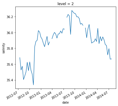
However, it is often much more powerful to use xarray’s .sel() method to use label-based indexing.
argo.salinity.sel(level=2).plot()
[<matplotlib.lines.Line2D at 0x7f6a9b38f520>]
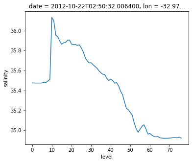
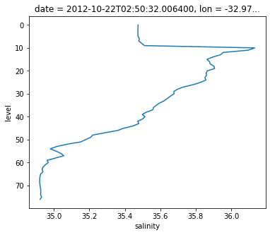
argo.salinity.sel(date='2012-10-22').plot(y='level', yincrease=False)
[<matplotlib.lines.Line2D at 0x7f6a9b44a2e0>]
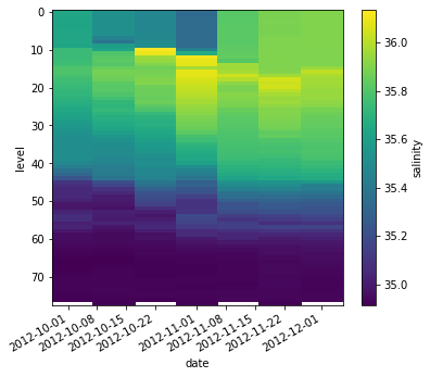
.sel() also supports slicing. Unfortunately we have to use a somewhat awkward syntax, but it still works.
argo.salinity.sel(date=slice('2012-10-01', '2012-12-01')).plot(yincrease=False)
<matplotlib.collections.QuadMesh at 0x7f6a9b354ee0>
.sel() also works on the whole Dataset
argo.sel(date='2012-10-22')
<xarray.Dataset>
Dimensions:      (date: 1, level: 78)
Coordinates:
  * level        (level) int64 0 1 2 3 4 5 6 7 8 ... 69 70 71 72 73 74 75 76 77
  * date         (date) datetime64[ns] 2012-10-22T02:50:32.006400
    lon          (date) float64 -32.97
    lat          (date) float64 44.13
Data variables:
    salinity     (level, date) float64 35.47 35.47 35.47 ... 34.93 34.92 nan
    temperature  (level, date) float64 17.13 17.13 17.13 ... 3.736 3.639 nan
pressure (level, date) float64 6.4 10.3 15.4 ... 1.9e+03 1.951e+03 nan- date: 1
- level: 78
- level(level)int640 1 2 3 4 5 6 ... 72 73 74 75 76 77
array([ 0, 1, 2, 3, 4, 5, 6, 7, 8, 9, 10, 11, 12, 13, 14, 15, 16, 17, 18, 19, 20, 21, 22, 23, 24, 25, 26, 27, 28, 29, 30, 31, 32, 33, 34, 35, 36, 37, 38, 39, 40, 41, 42, 43, 44, 45, 46, 47, 48, 49, 50, 51, 52, 53, 54, 55, 56, 57, 58, 59, 60, 61, 62, 63, 64, 65, 66, 67, 68, 69, 70, 71, 72, 73, 74, 75, 76, 77]) - date(date)datetime64[ns]2012-10-22T02:50:32.006400
array(['2012-10-22T02:50:32.006400000'], dtype='datetime64[ns]')
- lon(date)float64-32.97
array([-32.972])
- lat(date)float6444.13
array([44.13])
- salinity(level, date)float6435.47 35.47 35.47 ... 34.92 nan
array([[35.47483063], [35.47483063], [35.47383118], [35.47383118], [35.47383118], [35.47483063], [35.48183441], [35.47983551], [35.4948349 ], [35.51083755], [36.13380051], [36.09579849], [35.95479965], [35.93979645], [35.8958931 ], [35.86388397], [35.87788773], [35.88188934], [35.90379333], [35.9067955 ], ... [35.00975037], [34.96175385], [34.96775055], [34.95075226], [34.93775177], [34.93375015], [34.93775558], [34.9247551 ], [34.92175674], [34.91975403], [34.91975403], [34.91975403], [34.92176056], [34.92375946], [34.92575836], [34.92575836], [34.92475891], [34.93076324], [34.92176437], [ nan]]) - temperature(level, date)float6417.13 17.13 17.13 ... 3.639 nan
array([[17.13299942], [17.13199997], [17.13299942], [17.13400078], [17.13500023], [17.13500023], [17.13199997], [17.13400078], [17.11300087], [17.09700012], [16.67099953], [16.40099907], [15.76000023], [15.58600044], [15.35299969], [15.18299961], [15.15299988], [15.05799961], [15.04399967], [14.99300003], ... [ 5.04799986], [ 4.69399977], [ 4.61399984], [ 4.42500019], [ 4.30600023], [ 4.23099995], [ 4.19500017], [ 4.07600021], [ 4.0170002 ], [ 3.95000005], [ 3.92499995], [ 3.87899995], [ 3.86800003], [ 3.84500003], [ 3.8210001 ], [ 3.77800012], [ 3.73799992], [ 3.73600006], [ 3.63899994], [ nan]]) - pressure(level, date)float646.4 10.3 15.4 ... 1.951e+03 nan
array([[   6.4000001 ],
       [  10.30000019],
       [  15.39999962],
       [  21.        ],
       [  26.        ],
       [  30.20000076],
       [  35.40000153],
       [  40.79999924],
       [  44.79999924],
       [  51.29999924],
       [  60.20000076],
       [  71.        ],
       [  80.59999847],
       [  91.        ],
       [ 100.80000305],
       [ 110.90000153],
       [ 121.09999847],
       [ 130.8999939 ],
       [ 140.69999695],
       [ 150.80000305],
...
       [1050.        ],
       [1100.59997559],
       [1150.5       ],
       [1200.40002441],
       [1250.69995117],
       [1300.40002441],
       [1350.40002441],
       [1400.90002441],
       [1447.90002441],
       [1500.80004883],
       [1550.40002441],
       [1600.90002441],
       [1650.09997559],
       [1700.40002441],
       [1750.5       ],
       [1800.80004883],
       [1850.69995117],
       [1900.5       ],
       [1950.80004883],
       [          nan]])
Computation
Xarray DataArrays and Datasets work seamlessly with arithmetic operators and numpy array functions.
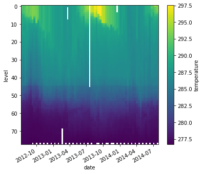
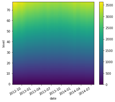
temp_kelvin = argo.temperature + 273.15
temp_kelvin.plot(yincrease=False)
<matplotlib.collections.QuadMesh at 0x7f6a9b25da60>
We can also combine multiple xarray datasets in arithemtic operations
g = 9.8
buoyancy = g * (2e-4 * argo.temperature - 7e-4 * argo.salinity)
buoyancy.plot(yincrease=False)
<matplotlib.collections.QuadMesh at 0x7f6a9b18ca90>
Broadcasting
Broadcasting arrays in numpy is a nightmare. It is much easier when the data axes are labeled!
This is a useless calculation, but it illustrates how perfoming an operation on arrays with differenty coordinates will result in automatic broadcasting
level_times_lat = argo.level * argo.lat
level_times_lat
<xarray.DataArray (level: 78, date: 75)>
array([[   0.   ,    0.   ,    0.   , ...,    0.   ,    0.   ,    0.   ],
       [  47.187,   46.716,   46.45 , ...,   42.601,   42.457,   42.379],
       [  94.374,   93.432,   92.9  , ...,   85.202,   84.914,   84.758],
       ...,
       [3539.025, 3503.7  , 3483.75 , ..., 3195.075, 3184.275, 3178.425],
       [3586.212, 3550.416, 3530.2  , ..., 3237.676, 3226.732, 3220.804],
       [3633.399, 3597.132, 3576.65 , ..., 3280.277, 3269.189, 3263.183]])
Coordinates:
  * level    (level) int64 0 1 2 3 4 5 6 7 8 9 ... 68 69 70 71 72 73 74 75 76 77
  * date     (date) datetime64[ns] 2012-07-13T22:33:06.019200 ... 2014-07-24T...
    lon      (date) float64 -39.13 -37.28 -36.9 -36.89 ... -33.83 -34.11 -34.38
lat (date) float64 47.19 46.72 46.45 46.23 ... 42.72 42.6 42.46 42.38- level: 78
- date: 75
- 0.0 0.0 0.0 0.0 0.0 ... 3.29e+03 3.28e+03 3.269e+03 3.263e+03
array([[ 0. , 0. , 0. , ..., 0. , 0. , 0. ], [ 47.187, 46.716, 46.45 , ..., 42.601, 42.457, 42.379], [ 94.374, 93.432, 92.9 , ..., 85.202, 84.914, 84.758], ..., [3539.025, 3503.7 , 3483.75 , ..., 3195.075, 3184.275, 3178.425], [3586.212, 3550.416, 3530.2 , ..., 3237.676, 3226.732, 3220.804], [3633.399, 3597.132, 3576.65 , ..., 3280.277, 3269.189, 3263.183]]) - level(level)int640 1 2 3 4 5 6 ... 72 73 74 75 76 77
array([ 0, 1, 2, 3, 4, 5, 6, 7, 8, 9, 10, 11, 12, 13, 14, 15, 16, 17, 18, 19, 20, 21, 22, 23, 24, 25, 26, 27, 28, 29, 30, 31, 32, 33, 34, 35, 36, 37, 38, 39, 40, 41, 42, 43, 44, 45, 46, 47, 48, 49, 50, 51, 52, 53, 54, 55, 56, 57, 58, 59, 60, 61, 62, 63, 64, 65, 66, 67, 68, 69, 70, 71, 72, 73, 74, 75, 76, 77]) - date(date)datetime64[ns]2012-07-13T22:33:06.019200 ... 2...
array(['2012-07-13T22:33:06.019200000', '2012-07-23T22:54:59.990400000', '2012-08-02T22:55:52.003200000', '2012-08-12T23:08:59.971200000', '2012-08-22T23:29:01.968000000', '2012-09-01T23:17:38.976000000', '2012-09-12T02:59:18.960000000', '2012-09-21T23:18:37.036800000', '2012-10-02T03:00:17.971200000', '2012-10-11T23:13:27.984000000', '2012-10-22T02:50:32.006400000', '2012-10-31T23:36:39.974400000', '2012-11-11T02:40:46.041600000', '2012-11-20T23:08:29.990400000', '2012-12-01T02:47:51.993600000', '2012-12-10T23:23:16.972800000', '2012-12-21T02:58:48.979200000', '2012-12-30T23:07:23.030400000', '2013-01-10T02:56:43.008000000', '2013-01-19T23:24:26.956800000', '2013-01-30T02:43:53.011200000', '2013-02-08T23:15:27.043200000', '2013-02-19T01:12:50.976000000', '2013-02-28T23:07:13.008000000', '2013-03-11T02:43:30.979200000', '2013-03-20T23:17:22.992000000', '2013-03-31T01:50:38.025600000', '2013-04-09T23:19:07.968000000', '2013-04-20T02:53:29.990400000', '2013-04-29T23:28:33.024000000', '2013-05-10T02:50:18.009600000', '2013-05-19T23:21:05.990400000', '2013-05-30T02:50:30.969600000', '2013-06-08T23:32:49.027200000', '2013-06-19T03:42:51.004800000', '2013-06-28T23:32:16.022400000', '2013-07-09T03:28:30.979199999', '2013-07-18T23:33:57.974400000', '2013-07-29T03:15:42.019200000', '2013-08-07T23:25:02.035200000', '2013-08-18T01:47:44.966400000', '2013-08-28T03:02:59.020800000', '2013-09-07T03:03:51.984000000', '2013-09-16T23:32:07.987200000', '2013-09-27T04:08:27.974400000', '2013-10-06T23:25:39.964800000', '2013-10-17T02:55:50.995200000', '2013-10-27T03:45:47.001600000', '2013-11-06T01:14:52.022400000', '2013-11-16T03:29:54.009600000', '2013-11-26T03:03:56.995200000', '2013-12-05T23:33:59.011200000', '2013-12-16T02:58:01.977600000', '2013-12-25T23:22:43.017600000', '2014-01-05T02:52:06.009600000', '2014-01-14T23:41:18.009600000', '2014-01-25T03:00:43.977600000', '2014-02-03T23:29:13.977600000', '2014-02-14T02:50:11.961600000', '2014-02-23T23:03:21.974400000', '2014-03-06T02:58:03.964800000', '2014-03-15T23:10:28.012800000', '2014-03-26T02:51:22.032000000', '2014-04-04T23:25:58.972800000', '2014-04-15T03:00:45.964800000', '2014-04-24T23:24:40.003200000', '2014-05-05T02:56:22.012800000', '2014-05-15T00:10:06.009600000', '2014-05-25T03:02:43.036800000', '2014-06-03T23:34:53.961600000', '2014-06-14T03:01:23.980800000', '2014-06-23T23:24:31.968000000', '2014-07-04T03:08:30.019200000', '2014-07-13T23:47:43.008000000', '2014-07-24T03:02:33.014400000'], dtype='datetime64[ns]') - lon(date)float64-39.13 -37.28 ... -34.11 -34.38
array([-39.13 , -37.282, -36.9 , -36.89 , -37.053, -36.658, -35.963, -35.184, -34.462, -33.784, -32.972, -32.546, -32.428, -32.292, -32.169, -31.998, -31.824, -31.624, -31.433, -31.312, -31.107, -31.147, -31.044, -31.14 , -31.417, -31.882, -32.145, -32.487, -32.537, -32.334, -32.042, -31.892, -31.861, -31.991, -31.883, -31.89 , -31.941, -31.889, -31.724, -31.412, -31.786, -31.561, -31.732, -31.553, -31.862, -32.389, -32.318, -32.19 , -32.224, -32.368, -32.306, -32.305, -32.65 , -33.093, -33.263, -33.199, -33.27 , -33.237, -33.221, -33.011, -32.844, -32.981, -32.784, -32.607, -32.87 , -33.196, -33.524, -33.956, -33.944, -33.71 , -33.621, -33.552, -33.828, -34.11 , -34.38 ]) - lat(date)float6447.19 46.72 46.45 ... 42.46 42.38
array([47.187, 46.716, 46.45 , 46.23 , 45.459, 44.833, 44.452, 44.839,
       44.956, 44.676, 44.13 , 43.644, 43.067, 42.662, 42.513, 42.454,
       42.396, 42.256, 42.089, 41.944, 41.712, 41.571, 41.596, 41.581,
       41.351, 41.032, 40.912, 40.792, 40.495, 40.383, 40.478, 40.672,
       41.032, 40.864, 40.651, 40.425, 40.228, 40.197, 40.483, 40.311,
       40.457, 40.463, 40.164, 40.047, 39.963, 40.122, 40.57 , 40.476,
       40.527, 40.589, 40.749, 40.993, 41.162, 41.237, 41.448, 41.65 ,
       42.053, 42.311, 42.096, 41.683, 41.661, 41.676, 42.018, 42.395,
       42.532, 42.558, 42.504, 42.63 , 42.934, 42.952, 42.777, 42.722,
       42.601, 42.457, 42.379])
level_times_lat.plot()
<matplotlib.collections.QuadMesh at 0x7f6a9b0b65b0>
Reductions
Just like in numpy, we can reduce xarray DataArrays along any number of axes:
argo.temperature.mean(axis=0).dims
('date',)
argo.temperature.mean(axis=1).dims
('level',)
However, rather than performing reductions on axes (as in numpy), we can perform them on dimensions. This turns out to be a huge convenience
argo_mean = argo.mean(dim='date')
argo_mean
<xarray.Dataset>
Dimensions:      (level: 78)
Coordinates:
  * level        (level) int64 0 1 2 3 4 5 6 7 8 ... 69 70 71 72 73 74 75 76 77
Data variables:
    salinity     (level) float64 35.91 35.9 35.9 35.9 ... 34.94 34.94 34.93
    temperature  (level) float64 17.6 17.57 17.51 17.42 ... 3.789 3.73 3.662
pressure (level) float64 6.435 10.57 15.54 ... 1.95e+03 1.999e+03- level: 78
- level(level)int640 1 2 3 4 5 6 ... 72 73 74 75 76 77
array([ 0,  1,  2,  3,  4,  5,  6,  7,  8,  9, 10, 11, 12, 13, 14, 15, 16, 17,
       18, 19, 20, 21, 22, 23, 24, 25, 26, 27, 28, 29, 30, 31, 32, 33, 34, 35,
       36, 37, 38, 39, 40, 41, 42, 43, 44, 45, 46, 47, 48, 49, 50, 51, 52, 53,
       54, 55, 56, 57, 58, 59, 60, 61, 62, 63, 64, 65, 66, 67, 68, 69, 70, 71,
       72, 73, 74, 75, 76, 77])
- salinity(level)float6435.91 35.9 35.9 ... 34.94 34.93
array([35.9063218 , 35.90223138, 35.90313435, 35.90173139, 35.90544583, 35.9100359 , 35.90946015, 35.91343146, 35.91967712, 35.92615988, 35.93195456, 35.94055356, 35.94091596, 35.93905366, 35.93931069, 35.93786745, 35.93525794, 35.93118039, 35.92534328, 35.91652257, 35.90671895, 35.89617843, 35.88888019, 35.8789927 , 35.86946183, 35.8598671 , 35.85061713, 35.84211978, 35.83150467, 35.81969395, 35.80945061, 35.80092265, 35.79078674, 35.77886525, 35.76833627, 35.75838795, 35.74923783, 35.73923559, 35.73000444, 35.71877237, 35.68864513, 35.65607159, 35.62678265, 35.59231774, 35.56205662, 35.45401408, 35.41392634, 35.3810557 , 35.34845245, 35.31531555, 35.28392568, 35.26568334, 35.2389473 , 35.21583745, 35.19686081, 35.18231257, 35.1648436 , 35.15073542, 35.12509338, 35.10155869, 35.08199799, 35.06317012, 35.0490097 , 35.03678253, 35.02174266, 35.01135579, 35.00212936, 34.99386297, 34.98810328, 34.98008094, 34.97214884, 34.96517645, 34.95664983, 34.9507985 , 34.9465696 , 34.94198907, 34.93844852, 34.93290652]) - temperature(level)float6417.6 17.57 17.51 ... 3.73 3.662
array([17.60172602, 17.57223609, 17.5145833 , 17.42326395, 17.24943838, 17.03730134, 16.76787661, 16.44609588, 16.17439195, 16.04501356, 15.65827023, 15.4607296 , 15.26114862, 15.12489191, 14.99133783, 14.90160808, 14.81990544, 14.74535139, 14.66822971, 14.585027 , 14.49732434, 14.41904053, 14.35412163, 14.27102702, 14.19081082, 14.11487838, 14.04347293, 13.98067566, 13.90994595, 13.83274319, 13.76139196, 13.69836479, 13.62335132, 13.54185131, 13.46647295, 13.39395946, 13.32541891, 13.25205403, 13.18131082, 13.10233782, 12.89268916, 12.67795943, 12.4649189 , 12.2178513 , 11.98270268, 11.1281081 , 10.80430666, 10.49702667, 10.1749066 , 9.83453334, 9.48625332, 9.19793334, 8.66010666, 8.12324001, 7.60221333, 7.15289333, 6.74250667, 6.39543999, 6.04598667, 5.74538665, 5.48913333, 5.26604001, 5.08768 , 4.93479998, 4.77769334, 4.65368 , 4.54237334, 4.44274664, 4.35933333, 4.2653784 , 4.17290539, 4.08902703, 3.99864865, 3.92163514, 3.85617567, 3.78916217, 3.72950001, 3.66207691]) - pressure(level)float646.435 10.57 ... 1.95e+03 1.999e+03
array([   6.43466671,   10.56891882,   15.54246568,   20.46301361,
         25.42567552,   30.44459441,   35.44324375,   40.4391894 ,
         45.40810832,   50.37837879,   60.47297323,   70.48378413,
         80.40270347,   90.48243311,  100.51216311,  110.46081151,
        120.52702795,  130.49459282,  140.51216064,  150.40540376,
        160.40810559,  170.36216035,  180.41080949,  190.4108097 ,
        200.39999761,  210.34729499,  220.32026858,  230.31351224,
        240.28918808,  250.41486297,  260.39999843,  270.36891752,
        280.42432136,  290.42297075,  300.4229691 ,  310.46351087,
        320.50675346,  330.5297266 ,  340.41891521,  350.49729383,
        375.41080867,  400.3797294 ,  425.29864626,  450.38378205,
        475.30675403,  550.47703016,  575.68400146,  600.42400716,
        625.30800456,  650.34533773,  675.33333984,  700.37067546,
        750.42400716,  800.36666992,  850.38534017,  900.4613387 ,
        950.45067383, 1000.38534261, 1050.38534668, 1100.45734212,
       1150.45201335, 1200.40534505, 1250.25067383, 1300.49467773,
       1350.40268392, 1400.41734538, 1450.25734212, 1500.40267253,
       1550.46401367, 1600.44055011, 1650.34595056, 1700.42163251,
       1750.42299013, 1800.35677358, 1850.33379467, 1900.20676401,
       1950.20946771, 1999.28975423])
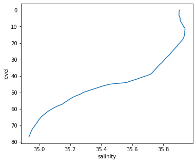
argo_mean.salinity.plot(y='level', yincrease=False)
[<matplotlib.lines.Line2D at 0x7f6a9b004cd0>]
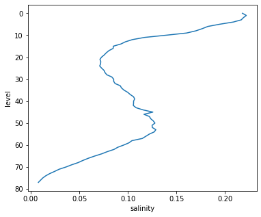
argo_std = argo.std(dim='date')
argo_std.salinity.plot(y='level', yincrease=False)
[<matplotlib.lines.Line2D at 0x7f6a9afec0a0>]
Loading Data from netCDF Files
As we already saw, NetCDF (Network Common Data Format) is the most widely used format for distributing geoscience data. NetCDF is maintained by the Unidata organization.
Below we quote from the NetCDF website:
NetCDF (network Common Data Form) is a set of interfaces for array-oriented data access and a freely distributed collection of data access libraries for C, Fortran, C++, Java, and other languages. The netCDF libraries support a machine-independent format for representing scientific data. Together, the interfaces, libraries, and format support the creation, access, and sharing of scientific data.
NetCDF data is:
Self-Describing. A netCDF file includes information about the data it contains.
Portable. A netCDF file can be accessed by computers with different ways of storing integers, characters, and floating-point numbers.
Scalable. A small subset of a large dataset may be accessed efficiently.
Appendable. Data may be appended to a properly structured netCDF file without copying the dataset or redefining its structure.
Sharable. One writer and multiple readers may simultaneously access the same netCDF file.
Archivable. Access to all earlier forms of netCDF data will be supported by current and future versions of the software.
See also
Xarray was designed to make reading netCDF files in python as easy, powerful, and flexible as possible. (See xarray netCDF docs for more details.)
Below we load one the previous eReefs data from the AIMS server.
month = 3
year = 2020
netCDF_datestr = str(year)+'-'+format(month, '02')

# GBR4 HYDRO
inputFile = "http://thredds.ereefs.aims.gov.au/thredds/dodsC/s3://aims-ereefs-public-prod/derived/ncaggregate/ereefs/gbr4_v2/daily-monthly/EREEFS_AIMS-CSIRO_gbr4_v2_hydro_daily-monthly-"+netCDF_datestr+".nc"

ds = xr.open_dataset(inputFile)
ds
<xarray.Dataset>
Dimensions:      (k: 17, latitude: 723, longitude: 491, time: 31)
Coordinates:
    zc           (k) float64 -145.0 -120.0 -103.0 -88.0 ... -5.55 -3.0 -1.5 -0.5
  * time         (time) datetime64[ns] 2020-02-29T14:00:00 ... 2020-03-30T14:...
  * latitude     (latitude) float64 -28.7 -28.67 -28.64 ... -7.096 -7.066 -7.036
  * longitude    (longitude) float64 142.2 142.2 142.2 ... 156.8 156.8 156.9
Dimensions without coordinates: k
Data variables:
    mean_cur     (time, k, latitude, longitude) float32 ...
    salt         (time, k, latitude, longitude) float32 ...
    temp         (time, k, latitude, longitude) float32 ...
    u            (time, k, latitude, longitude) float32 ...
    v            (time, k, latitude, longitude) float32 ...
    mean_wspeed  (time, latitude, longitude) float32 ...
    eta          (time, latitude, longitude) float32 ...
    wspeed_u     (time, latitude, longitude) float32 ...
    wspeed_v     (time, latitude, longitude) float32 ...
Attributes: (12/19)
    Conventions:                     CF-1.0
    Run_ID:                          2.1
    _CoordSysBuilder:                ucar.nc2.dataset.conv.CF1Convention
    aims_ncaggregate_buildDate:      2020-08-21T15:38:56+10:00
    aims_ncaggregate_datasetId:      products__ncaggregate__ereefs__gbr4_v2__...
    aims_ncaggregate_firstDate:      2020-03-01T00:00:00+10:00
    ...                              ...
    paramfile:                       in.prm
    paramhead:                       GBR 4km resolution grid
    technical_guide_link:            https://eatlas.org.au/pydio/public/aims-...
    technical_guide_publish_date:    2020-08-18
    title:                           eReefs AIMS-CSIRO GBR4 Hydrodynamic v2 d...
DODS_EXTRA.Unlimited_Dimension: time- k: 17
- latitude: 723
- longitude: 491
- time: 31
- zc(k)float64...
- positive :
- up
- coordinate_type :
- Z
- units :
- m
- long_name :
- Z coordinate
- axis :
- Z
- _CoordinateAxisType :
- Height
- _CoordinateZisPositive :
- up
array([-145. , -120. , -103. , -88. , -73. , -60. , -49. , -39.5 , -31. , -23.75, -17.75, -12.75, -8.8 , -5.55, -3. , -1.5 , -0.5 ]) - time(time)datetime64[ns]2020-02-29T14:00:00 ... 2020-03-...
- long_name :
- Time
- standard_name :
- time
- coordinate_type :
- time
- _CoordinateAxisType :
- Time
- _ChunkSizes :
- 1024
array(['2020-02-29T14:00:00.000000000', '2020-03-01T14:00:00.000000000', '2020-03-02T14:00:00.000000000', '2020-03-03T14:00:00.000000000', '2020-03-04T14:00:00.000000000', '2020-03-05T14:00:00.000000000', '2020-03-06T14:00:00.000000000', '2020-03-07T14:00:00.000000000', '2020-03-08T14:00:00.000000000', '2020-03-09T14:00:00.000000000', '2020-03-10T14:00:00.000000000', '2020-03-11T14:00:00.000000000', '2020-03-12T14:00:00.000000000', '2020-03-13T14:00:00.000000000', '2020-03-14T14:00:00.000000000', '2020-03-15T14:00:00.000000000', '2020-03-16T14:00:00.000000000', '2020-03-17T14:00:00.000000000', '2020-03-18T14:00:00.000000000', '2020-03-19T14:00:00.000000000', '2020-03-20T14:00:00.000000000', '2020-03-21T14:00:00.000000000', '2020-03-22T14:00:00.000000000', '2020-03-23T14:00:00.000000000', '2020-03-24T14:00:00.000000000', '2020-03-25T14:00:00.000000000', '2020-03-26T14:00:00.000000000', '2020-03-27T14:00:00.000000000', '2020-03-28T14:00:00.000000000', '2020-03-29T14:00:00.000000000', '2020-03-30T14:00:00.000000000'], dtype='datetime64[ns]') - latitude(latitude)float64-28.7 -28.67 ... -7.066 -7.036
- long_name :
- Latitude
- standard_name :
- latitude
- units :
- degrees_north
- coordinate_type :
- latitude
- projection :
- geographic
- _CoordinateAxisType :
- Lat
array([-28.696022, -28.666022, -28.636022, ..., -7.096022, -7.066022, -7.036022]) - longitude(longitude)float64142.2 142.2 142.2 ... 156.8 156.9
- standard_name :
- longitude
- long_name :
- Longitude
- units :
- degrees_east
- coordinate_type :
- longitude
- projection :
- geographic
- _CoordinateAxisType :
- Lon
array([142.168788, 142.198788, 142.228788, ..., 156.808788, 156.838788,
       156.868788])
- mean_cur(time, k, latitude, longitude)float32...
- substanceOrTaxon_id :
- http://environment.data.gov.au/def/feature/ocean_current
- units :
- ms-1
- medium_id :
- http://environment.data.gov.au/def/feature/ocean
- unit_id :
- http://qudt.org/vocab/unit#MeterPerSecond
- short_name :
- mean_cur
- aggregation :
- mean_speed
- standard_name :
- mean_current_speed
- long_name :
- mean_current_speed
- _ChunkSizes :
- [ 1 1 133 491]
[187081311 values with dtype=float32]
- salt(time, k, latitude, longitude)float32...
- substanceOrTaxon_id :
- http://sweet.jpl.nasa.gov/2.2/matrWater.owl#SaltWater
- scaledQuantityKind_id :
- http://environment.data.gov.au/def/property/practical_salinity
- short_name :
- salt
- aggregation :
- Daily
- units :
- PSU
- medium_id :
- http://environment.data.gov.au/def/feature/ocean
- unit_id :
- http://environment.data.gov.au/water/quality/def/unit/PSU
- long_name :
- Salinity
- _ChunkSizes :
- [ 1 1 133 491]
[187081311 values with dtype=float32]
- temp(time, k, latitude, longitude)float32...
- substanceOrTaxon_id :
- http://sweet.jpl.nasa.gov/2.2/matrWater.owl#SaltWater
- scaledQuantityKind_id :
- http://environment.data.gov.au/def/property/sea_water_temperature
- short_name :
- temp
- aggregation :
- Daily
- units :
- degrees C
- medium_id :
- http://environment.data.gov.au/def/feature/ocean
- unit_id :
- http://qudt.org/vocab/unit#DegreeCelsius
- long_name :
- Temperature
- _ChunkSizes :
- [ 1 1 133 491]
[187081311 values with dtype=float32]
- u(time, k, latitude, longitude)float32...
- vector_components :
- u v
- substanceOrTaxon_id :
- http://environment.data.gov.au/def/feature/ocean_current
- scaledQuantityKind_id :
- http://environment.data.gov.au/def/property/sea_water_velocity_eastward
- short_name :
- u
- vector_name :
- Currents
- standard_name :
- eastward_sea_water_velocity
- aggregation :
- Daily
- units :
- ms-1
- medium_id :
- http://environment.data.gov.au/def/feature/ocean
- unit_id :
- http://qudt.org/vocab/unit#MeterPerSecond
- long_name :
- Eastward current
- _ChunkSizes :
- [ 1 1 133 491]
[187081311 values with dtype=float32]
- v(time, k, latitude, longitude)float32...
- vector_components :
- u v
- substanceOrTaxon_id :
- http://environment.data.gov.au/def/feature/ocean_current
- scaledQuantityKind_id :
- http://environment.data.gov.au/def/property/sea_water_velocity_northward
- short_name :
- v
- vector_name :
- Currents
- standard_name :
- northward_sea_water_velocity
- aggregation :
- Daily
- units :
- ms-1
- medium_id :
- http://environment.data.gov.au/def/feature/ocean
- unit_id :
- http://qudt.org/vocab/unit#MeterPerSecond
- long_name :
- Northward current
- _ChunkSizes :
- [ 1 1 133 491]
[187081311 values with dtype=float32]
- mean_wspeed(time, latitude, longitude)float32...
- units :
- ms-1
- short_name :
- mean_wspeed
- aggregation :
- mean_speed
- standard_name :
- mean_wind_speed
- long_name :
- mean_wind_speed
- _ChunkSizes :
- [ 1 133 491]
[11004783 values with dtype=float32]
- eta(time, latitude, longitude)float32...
- substanceOrTaxon_id :
- http://environment.data.gov.au/def/feature/ocean_near_surface
- scaledQuantityKind_id :
- http://environment.data.gov.au/def/property/sea_surface_elevation
- short_name :
- eta
- standard_name :
- sea_surface_height_above_sea_level
- aggregation :
- Daily
- units :
- metre
- positive :
- up
- medium_id :
- http://environment.data.gov.au/def/feature/ocean
- unit_id :
- http://qudt.org/vocab/unit#Meter
- long_name :
- Surface elevation
- _ChunkSizes :
- [ 1 133 491]
[11004783 values with dtype=float32]
- wspeed_u(time, latitude, longitude)float32...
- short_name :
- wspeed_u
- aggregation :
- Daily
- units :
- ms-1
- long_name :
- eastward_wind
- _ChunkSizes :
- [ 1 133 491]
[11004783 values with dtype=float32]
- wspeed_v(time, latitude, longitude)float32...
- short_name :
- wspeed_v
- aggregation :
- Daily
- units :
- ms-1
- long_name :
- northward_wind
- _ChunkSizes :
- [ 1 133 491]
[11004783 values with dtype=float32]
- Conventions :
- CF-1.0
- Run_ID :
- 2.1
- _CoordSysBuilder :
- ucar.nc2.dataset.conv.CF1Convention
- aims_ncaggregate_buildDate :
- 2020-08-21T15:38:56+10:00
- aims_ncaggregate_datasetId :
- products__ncaggregate__ereefs__gbr4_v2__daily-monthly/EREEFS_AIMS-CSIRO_gbr4_v2_hydro_daily-monthly-2020-03
- aims_ncaggregate_firstDate :
- 2020-03-01T00:00:00+10:00
- aims_ncaggregate_inputs :
- [products__ncaggregate__ereefs__gbr4_v2__raw/EREEFS_AIMS-CSIRO_gbr4_v2_hydro_raw_2020-03::MD5:36889e7fad180571a4a68ccca19c7384]
- aims_ncaggregate_lastDate :
- 2020-03-31T00:00:00+10:00
- description :
- Aggregation of raw hourly input data (from eReefs AIMS-CSIRO GBR4 Hydrodynamic v2 subset) to daily means. Also calculates mean magnitude of wind and ocean current speeds. Data is regridded from curvilinear (per input data) to rectilinear via inverse weighted distance from up to 4 closest cells.
- ems_version :
- v1.0 rev(5996)
- hasVocab :
- 1
- history :
- 2020-08-20T15:04:55+10:00: vendor: AIMS; processing: None summaries 2020-08-21T15:38:56+10:00: vendor: AIMS; processing: Daily summaries
- metadata_link :
- https://eatlas.org.au/data/uuid/350aed53-ae0f-436e-9866-d34db7f04d2e
- paramfile :
- in.prm
- paramhead :
- GBR 4km resolution grid
- technical_guide_link :
- https://eatlas.org.au/pydio/public/aims-ereefs-platform-technical-guide-to-derived-products-from-csiro-ereefs-models-pdf
- technical_guide_publish_date :
- 2020-08-18
- title :
- eReefs AIMS-CSIRO GBR4 Hydrodynamic v2 daily aggregation
- DODS_EXTRA.Unlimited_Dimension :
- time
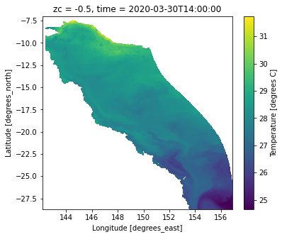
ds.temp.isel(time=-1,k=-1).plot()
<matplotlib.collections.QuadMesh at 0x7f6a9a738bb0>
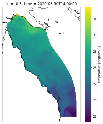
Let’s use Cartopy…
import cartopy.crs as ccrs

fig = plt.figure(figsize=[6, 7])
ax = fig.add_subplot(1, 1, 1, projection=ccrs.PlateCarree())

ds.temp.isel(time=-1,k=-1).plot(
    transform=ccrs.PlateCarree()
)

ax.coastlines()
<cartopy.mpl.feature_artist.FeatureArtist at 0x7f6a8dfb7ee0>
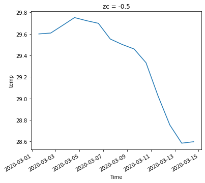
ds_slice = ds.sel(time=slice('2020-03-01', '2020-03-14'),k=-1)
ds_slice
<xarray.Dataset>
Dimensions:      (latitude: 723, longitude: 491, time: 14)
Coordinates:
    zc           float64 -0.5
  * time         (time) datetime64[ns] 2020-03-01T14:00:00 ... 2020-03-14T14:...
  * latitude     (latitude) float64 -28.7 -28.67 -28.64 ... -7.096 -7.066 -7.036
  * longitude    (longitude) float64 142.2 142.2 142.2 ... 156.8 156.8 156.9
Data variables:
    mean_cur     (time, latitude, longitude) float32 ...
    salt         (time, latitude, longitude) float32 ...
    temp         (time, latitude, longitude) float32 ...
    u            (time, latitude, longitude) float32 ...
    v            (time, latitude, longitude) float32 ...
    mean_wspeed  (time, latitude, longitude) float32 ...
    eta          (time, latitude, longitude) float32 ...
    wspeed_u     (time, latitude, longitude) float32 ...
    wspeed_v     (time, latitude, longitude) float32 ...
Attributes: (12/19)
    Conventions:                     CF-1.0
    Run_ID:                          2.1
    _CoordSysBuilder:                ucar.nc2.dataset.conv.CF1Convention
    aims_ncaggregate_buildDate:      2020-08-21T15:38:56+10:00
    aims_ncaggregate_datasetId:      products__ncaggregate__ereefs__gbr4_v2__...
    aims_ncaggregate_firstDate:      2020-03-01T00:00:00+10:00
    ...                              ...
    paramfile:                       in.prm
    paramhead:                       GBR 4km resolution grid
    technical_guide_link:            https://eatlas.org.au/pydio/public/aims-...
    technical_guide_publish_date:    2020-08-18
    title:                           eReefs AIMS-CSIRO GBR4 Hydrodynamic v2 d...
DODS_EXTRA.Unlimited_Dimension: time- latitude: 723
- longitude: 491
- time: 14
- zc()float64-0.5
- positive :
- up
- coordinate_type :
- Z
- units :
- m
- long_name :
- Z coordinate
- axis :
- Z
- _CoordinateAxisType :
- Height
- _CoordinateZisPositive :
- up
array(-0.5)
- time(time)datetime64[ns]2020-03-01T14:00:00 ... 2020-03-...
- long_name :
- Time
- standard_name :
- time
- coordinate_type :
- time
- _CoordinateAxisType :
- Time
- _ChunkSizes :
- 1024
array(['2020-03-01T14:00:00.000000000', '2020-03-02T14:00:00.000000000', '2020-03-03T14:00:00.000000000', '2020-03-04T14:00:00.000000000', '2020-03-05T14:00:00.000000000', '2020-03-06T14:00:00.000000000', '2020-03-07T14:00:00.000000000', '2020-03-08T14:00:00.000000000', '2020-03-09T14:00:00.000000000', '2020-03-10T14:00:00.000000000', '2020-03-11T14:00:00.000000000', '2020-03-12T14:00:00.000000000', '2020-03-13T14:00:00.000000000', '2020-03-14T14:00:00.000000000'], dtype='datetime64[ns]') - latitude(latitude)float64-28.7 -28.67 ... -7.066 -7.036
- long_name :
- Latitude
- standard_name :
- latitude
- units :
- degrees_north
- coordinate_type :
- latitude
- projection :
- geographic
- _CoordinateAxisType :
- Lat
array([-28.696022, -28.666022, -28.636022, ..., -7.096022, -7.066022, -7.036022]) - longitude(longitude)float64142.2 142.2 142.2 ... 156.8 156.9
- standard_name :
- longitude
- long_name :
- Longitude
- units :
- degrees_east
- coordinate_type :
- longitude
- projection :
- geographic
- _CoordinateAxisType :
- Lon
array([142.168788, 142.198788, 142.228788, ..., 156.808788, 156.838788,
       156.868788])
- mean_cur(time, latitude, longitude)float32...
- substanceOrTaxon_id :
- http://environment.data.gov.au/def/feature/ocean_current
- units :
- ms-1
- medium_id :
- http://environment.data.gov.au/def/feature/ocean
- unit_id :
- http://qudt.org/vocab/unit#MeterPerSecond
- short_name :
- mean_cur
- aggregation :
- mean_speed
- standard_name :
- mean_current_speed
- long_name :
- mean_current_speed
- _ChunkSizes :
- [ 1 1 133 491]
[4969902 values with dtype=float32]
- salt(time, latitude, longitude)float32...
- substanceOrTaxon_id :
- http://sweet.jpl.nasa.gov/2.2/matrWater.owl#SaltWater
- scaledQuantityKind_id :
- http://environment.data.gov.au/def/property/practical_salinity
- short_name :
- salt
- aggregation :
- Daily
- units :
- PSU
- medium_id :
- http://environment.data.gov.au/def/feature/ocean
- unit_id :
- http://environment.data.gov.au/water/quality/def/unit/PSU
- long_name :
- Salinity
- _ChunkSizes :
- [ 1 1 133 491]
[4969902 values with dtype=float32]
- temp(time, latitude, longitude)float32...
- substanceOrTaxon_id :
- http://sweet.jpl.nasa.gov/2.2/matrWater.owl#SaltWater
- scaledQuantityKind_id :
- http://environment.data.gov.au/def/property/sea_water_temperature
- short_name :
- temp
- aggregation :
- Daily
- units :
- degrees C
- medium_id :
- http://environment.data.gov.au/def/feature/ocean
- unit_id :
- http://qudt.org/vocab/unit#DegreeCelsius
- long_name :
- Temperature
- _ChunkSizes :
- [ 1 1 133 491]
[4969902 values with dtype=float32]
- u(time, latitude, longitude)float32...
- vector_components :
- u v
- substanceOrTaxon_id :
- http://environment.data.gov.au/def/feature/ocean_current
- scaledQuantityKind_id :
- http://environment.data.gov.au/def/property/sea_water_velocity_eastward
- short_name :
- u
- vector_name :
- Currents
- standard_name :
- eastward_sea_water_velocity
- aggregation :
- Daily
- units :
- ms-1
- medium_id :
- http://environment.data.gov.au/def/feature/ocean
- unit_id :
- http://qudt.org/vocab/unit#MeterPerSecond
- long_name :
- Eastward current
- _ChunkSizes :
- [ 1 1 133 491]
[4969902 values with dtype=float32]
- v(time, latitude, longitude)float32...
- vector_components :
- u v
- substanceOrTaxon_id :
- http://environment.data.gov.au/def/feature/ocean_current
- scaledQuantityKind_id :
- http://environment.data.gov.au/def/property/sea_water_velocity_northward
- short_name :
- v
- vector_name :
- Currents
- standard_name :
- northward_sea_water_velocity
- aggregation :
- Daily
- units :
- ms-1
- medium_id :
- http://environment.data.gov.au/def/feature/ocean
- unit_id :
- http://qudt.org/vocab/unit#MeterPerSecond
- long_name :
- Northward current
- _ChunkSizes :
- [ 1 1 133 491]
[4969902 values with dtype=float32]
- mean_wspeed(time, latitude, longitude)float32...
- units :
- ms-1
- short_name :
- mean_wspeed
- aggregation :
- mean_speed
- standard_name :
- mean_wind_speed
- long_name :
- mean_wind_speed
- _ChunkSizes :
- [ 1 133 491]
[4969902 values with dtype=float32]
- eta(time, latitude, longitude)float32...
- substanceOrTaxon_id :
- http://environment.data.gov.au/def/feature/ocean_near_surface
- scaledQuantityKind_id :
- http://environment.data.gov.au/def/property/sea_surface_elevation
- short_name :
- eta
- standard_name :
- sea_surface_height_above_sea_level
- aggregation :
- Daily
- units :
- metre
- positive :
- up
- medium_id :
- http://environment.data.gov.au/def/feature/ocean
- unit_id :
- http://qudt.org/vocab/unit#Meter
- long_name :
- Surface elevation
- _ChunkSizes :
- [ 1 133 491]
[4969902 values with dtype=float32]
- wspeed_u(time, latitude, longitude)float32...
- short_name :
- wspeed_u
- aggregation :
- Daily
- units :
- ms-1
- long_name :
- eastward_wind
- _ChunkSizes :
- [ 1 133 491]
[4969902 values with dtype=float32]
- wspeed_v(time, latitude, longitude)float32...
- short_name :
- wspeed_v
- aggregation :
- Daily
- units :
- ms-1
- long_name :
- northward_wind
- _ChunkSizes :
- [ 1 133 491]
[4969902 values with dtype=float32]
- Conventions :
- CF-1.0
- Run_ID :
- 2.1
- _CoordSysBuilder :
- ucar.nc2.dataset.conv.CF1Convention
- aims_ncaggregate_buildDate :
- 2020-08-21T15:38:56+10:00
- aims_ncaggregate_datasetId :
- products__ncaggregate__ereefs__gbr4_v2__daily-monthly/EREEFS_AIMS-CSIRO_gbr4_v2_hydro_daily-monthly-2020-03
- aims_ncaggregate_firstDate :
- 2020-03-01T00:00:00+10:00
- aims_ncaggregate_inputs :
- [products__ncaggregate__ereefs__gbr4_v2__raw/EREEFS_AIMS-CSIRO_gbr4_v2_hydro_raw_2020-03::MD5:36889e7fad180571a4a68ccca19c7384]
- aims_ncaggregate_lastDate :
- 2020-03-31T00:00:00+10:00
- description :
- Aggregation of raw hourly input data (from eReefs AIMS-CSIRO GBR4 Hydrodynamic v2 subset) to daily means. Also calculates mean magnitude of wind and ocean current speeds. Data is regridded from curvilinear (per input data) to rectilinear via inverse weighted distance from up to 4 closest cells.
- ems_version :
- v1.0 rev(5996)
- hasVocab :
- 1
- history :
- 2020-08-20T15:04:55+10:00: vendor: AIMS; processing: None summaries 2020-08-21T15:38:56+10:00: vendor: AIMS; processing: Daily summaries
- metadata_link :
- https://eatlas.org.au/data/uuid/350aed53-ae0f-436e-9866-d34db7f04d2e
- paramfile :
- in.prm
- paramhead :
- GBR 4km resolution grid
- technical_guide_link :
- https://eatlas.org.au/pydio/public/aims-ereefs-platform-technical-guide-to-derived-products-from-csiro-ereefs-models-pdf
- technical_guide_publish_date :
- 2020-08-18
- title :
- eReefs AIMS-CSIRO GBR4 Hydrodynamic v2 daily aggregation
- DODS_EXTRA.Unlimited_Dimension :
- time
ds_slice.temp.mean(dim=('longitude', 'latitude')).plot()
[<matplotlib.lines.Line2D at 0x7f6a8ce919d0>]