.ipynb .pdf

repository open issue suggest edit

Binder

Contents

Xarray maps

In this example, we will start exporting eReefs data using the Xarray library and do similar visualisation as the ones we did with Numpy.

Load the required Python libraries

First of all, load the necessary libraries. These are the ones we discussed previously:

• numpy

• matplotlib

• cartopy

• xarray

import os
import numpy as np
import xarray as xr

import cartopy
import cartopy.crs as ccrs
import cartopy.feature as cfeature
from cartopy.mpl.gridliner import LONGITUDE_FORMATTER, LATITUDE_FORMATTER
cartopy.config['data_dir'] = os.getenv('CARTOPY_DIR', cartopy.config.get('data_dir'))

import cmocean

from matplotlib import pyplot as plt
#%config InlineBackend.figure_format = 'retina'
plt.ion()  # To trigger the interactive inline mode

import warnings
warnings.filterwarnings("ignore", category=RuntimeWarning) 

Build multi-file dataset

We will use the open_mfdataset function from xArray to open multiple netCDF files into a single xarray Dataset.

We will query load the GBR4km dataset from the AIMS server, so let’s first define the base URL:

# For the bio dataset
base_url = "http://thredds.ereefs.aims.gov.au/thredds/dodsC/s3://aims-ereefs-public-prod/derived/ncaggregate/ereefs/GBR4_H2p0_B3p1_Cq3b_Dhnd/daily-monthly/EREEFS_AIMS-CSIRO_GBR4_H2p0_B3p1_Cq3b_Dhnd_bgc_daily-monthly-"

# For the hydro dataset
base_url2 = "http://thredds.ereefs.aims.gov.au/thredds/dodsC/s3://aims-ereefs-public-prod/derived/ncaggregate/ereefs/gbr4_v2/daily-monthly/EREEFS_AIMS-CSIRO_gbr4_v2_hydro_daily-monthly-"

For the sake of the demonstration, we will only use 1 month:

month_st = 1   # Starting month 
month_ed = 1   # Ending month 
year = 2018    # Year

# Based on the server the file naming convention 
biofiles = [f"{base_url}{year}-{month:02}.nc" for month in range(month_st, month_ed+1)]
hydrofiles = [f"{base_url2}{year}-{month:02}.nc" for month in range(month_st, month_ed+1)]

Loading dataset into xArray

Using xArray, we open these files into a Dataset:

ds_bio = xr.open_mfdataset(biofiles)
ds_hydro = xr.open_mfdataset(hydrofiles)

ds_bio

<xarray.Dataset>
Dimensions:          (k: 17, latitude: 723, longitude: 491, time: 31)
Coordinates:
    zc               (k) float64 dask.array<chunksize=(17,), meta=np.ndarray>
  * time             (time) datetime64[ns] 2018-01-01T02:00:00 ... 2018-01-31...
  * latitude         (latitude) float64 -28.7 -28.67 -28.64 ... -7.066 -7.036
  * longitude        (longitude) float64 142.2 142.2 142.2 ... 156.8 156.8 156.9
Dimensions without coordinates: k
Data variables: (12/101)
    alk              (time, k, latitude, longitude) float32 dask.array<chunksize=(31, 17, 723, 491), meta=np.ndarray>
    BOD              (time, k, latitude, longitude) float32 dask.array<chunksize=(31, 17, 723, 491), meta=np.ndarray>
    Chl_a_sum        (time, k, latitude, longitude) float32 dask.array<chunksize=(31, 17, 723, 491), meta=np.ndarray>
    CO32             (time, k, latitude, longitude) float32 dask.array<chunksize=(31, 17, 723, 491), meta=np.ndarray>
    DIC              (time, k, latitude, longitude) float32 dask.array<chunksize=(31, 17, 723, 491), meta=np.ndarray>
    DIN              (time, k, latitude, longitude) float32 dask.array<chunksize=(31, 17, 723, 491), meta=np.ndarray>
    ...               ...
    SGH_N            (time, latitude, longitude) float32 dask.array<chunksize=(31, 723, 491), meta=np.ndarray>
    SGH_N_pr         (time, latitude, longitude) float32 dask.array<chunksize=(31, 723, 491), meta=np.ndarray>
    SGHROOT_N        (time, latitude, longitude) float32 dask.array<chunksize=(31, 723, 491), meta=np.ndarray>
    SGROOT_N         (time, latitude, longitude) float32 dask.array<chunksize=(31, 723, 491), meta=np.ndarray>
    TSSM             (time, latitude, longitude) float32 dask.array<chunksize=(31, 723, 491), meta=np.ndarray>
    Zenith2D         (time, latitude, longitude) float32 dask.array<chunksize=(31, 723, 491), meta=np.ndarray>
Attributes: (12/20)
    Conventions:                     CF-1.0
    NCO:                             netCDF Operators version 4.7.7 (Homepage...
    RunID:                           2
    _CoordSysBuilder:                ucar.nc2.dataset.conv.CF1Convention
    aims_ncaggregate_buildDate:      2020-08-21T23:07:30+10:00
    aims_ncaggregate_datasetId:      products__ncaggregate__ereefs__GBR4_H2p0...
    ...                              ...
    paramfile:                       /home/bai155/EMS_solar2/gbr4_H2p0_B3p1_C...
    paramhead:                       eReefs 4 km grid. SOURCE Catchments with...
    technical_guide_link:            https://eatlas.org.au/pydio/public/aims-...
    technical_guide_publish_date:    2020-08-18
    title:                           eReefs AIMS-CSIRO GBR4 BioGeoChemical 3....
    DODS_EXTRA.Unlimited_Dimension:  time

Davies Reef position:

reef_lat = -18.82
reef_lon = 147.64

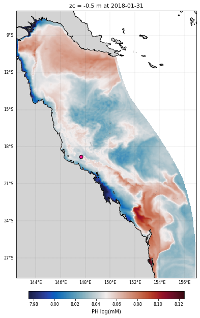
Plotting Xarray dataset

We will use the Xarray plot function.

See also

Check out this link to see how to use Xarray’s convenient matplotlib-backed plotting interface to visualize your datasets!

# Figure size
size = (9, 10)

# Color from cmocean
color = cmocean.cm.balance

# Defining the figure
fig = plt.figure(figsize=size, facecolor='w', edgecolor='k')

# Axes with Cartopy projection
ax = plt.axes(projection=ccrs.PlateCarree())
# and extent
ax.set_extent([142.4, 157, -7, -28.6], ccrs.PlateCarree())

# Plotting using Matplotlib 
# We plot the PH at the surface at the final recorded time interval
cf = ds_bio.PH.isel(time=-1,k=-1).plot( 
    transform=ccrs.PlateCarree(), cmap=color,
    vmin = 7.975, vmax = 8.125,
    add_colorbar=False
)

# Color bar
cbar = fig.colorbar(cf, ax=ax, fraction=0.027, pad=0.045, 
                    orientation="horizontal")
cbar.set_label(ds_bio.PH.long_name+' '+ds_bio.PH.units, rotation=0, 
               labelpad=5, fontsize=10)
cbar.ax.tick_params(labelsize=8)

# Title
plt.title('zc = '+str(ds_bio.zc.values.item(-1))+' m at '+str(ds_bio.coords['time'].values[-1])[:10],
          fontsize=11
         )

# Plot lat/lon grid 
gl = ax.gridlines(crs=ccrs.PlateCarree(), draw_labels=True,
                  linewidth=0.1, color='k', alpha=1, 
                  linestyle='--')
gl.top_labels = False
gl.right_labels = False
gl.xformatter = LONGITUDE_FORMATTER
gl.yformatter = LATITUDE_FORMATTER
gl.xlabel_style = {'size': 8}
gl.ylabel_style = {'size': 8} 

# Add map features with Cartopy 
ax.add_feature(cfeature.NaturalEarthFeature('physical', 'land', '10m', 
                                            edgecolor='face', 
                                            facecolor='lightgray'))
ax.coastlines(linewidth=1)

# Site Davies Reef
ax.scatter(reef_lon, reef_lat, c='deeppink', s=50, edgecolors='k', linewidth=1, transform=ccrs.PlateCarree())

plt.tight_layout()
plt.show()
fig.clear()
plt.close(fig)
plt.clf()

<Figure size 432x288 with 0 Axes>

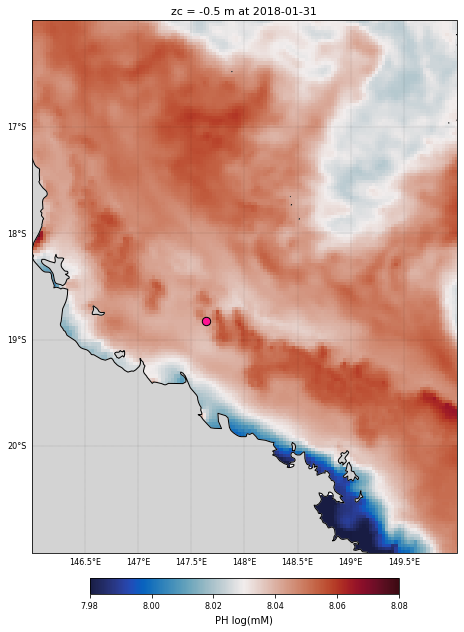
Clip the Dataset

To reduce the Dataset size we will clip the spatial extent based on longitudinal and latitudinal values.

This is easely done using the sel function with the slice method.

min_lon = 146     # lower left longitude
min_lat = -21     # lower left latitude
max_lon = 150     # upper right longitude
max_lat = -16     # upper right latitude

# Defining the boundaries
lon_bnds = [min_lon, max_lon]
lat_bnds = [min_lat, max_lat]

# Performing the reduction
ds_bio_clip = ds_bio.sel(latitude=slice(*lat_bnds), longitude=slice(*lon_bnds))
ds_hydro_clip = ds_hydro.sel(latitude=slice(*lat_bnds), longitude=slice(*lon_bnds))

Let’s plot the clipped region using the same approach as above:

# Figure size
size = (9, 10)

# Color from cmocean
color = cmocean.cm.balance

# Defining the figure
fig = plt.figure(figsize=size, facecolor='w', edgecolor='k')

# Axes with Cartopy projection
ax = plt.axes(projection=ccrs.PlateCarree())
# and extent
ax.set_extent([min_lon, max_lon, min_lat, max_lat], ccrs.PlateCarree())

# Plotting using Matplotlib 
# We plot the PH at the surface at the final recorded time interval
cf = ds_bio_clip.PH.isel(time=-1,k=-1).plot( 
    transform=ccrs.PlateCarree(), cmap=color,
    vmin = 7.98, vmax = 8.08,
    add_colorbar=False
)

# Color bar
cbar = fig.colorbar(cf, ax=ax, fraction=0.027, pad=0.045, 
                    orientation="horizontal")
cbar.set_label(ds_bio_clip.PH.long_name+' '+ds_bio_clip.PH.units, rotation=0, 
               labelpad=5, fontsize=10)
cbar.ax.tick_params(labelsize=8)

# Title
plt.title('zc = '+str(ds_bio_clip.zc.values.item(-1))+' m at '+
          str(ds_bio_clip.coords['time'].values[-1])[:10],
          fontsize=11
         )

# Plot lat/lon grid 
gl = ax.gridlines(crs=ccrs.PlateCarree(), draw_labels=True,
                  linewidth=0.1, color='k', alpha=1, 
                  linestyle='--')
gl.top_labels = False
gl.right_labels = False
gl.xformatter = LONGITUDE_FORMATTER
gl.yformatter = LATITUDE_FORMATTER
gl.xlabel_style = {'size': 8}
gl.ylabel_style = {'size': 8} 

# Add map features with Cartopy 
ax.add_feature(cfeature.NaturalEarthFeature('physical', 'land', '10m', 
                                            edgecolor='face', 
                                            facecolor='lightgray'))
ax.coastlines(linewidth=1)

# Site Davies Reef
ax.scatter(reef_lon, reef_lat, c='deeppink', s=70, edgecolors='k', 
           linewidth=1, transform=ccrs.PlateCarree())

plt.tight_layout()
plt.show()
fig.clear()
plt.close(fig)
plt.clf()

<Figure size 432x288 with 0 Axes>

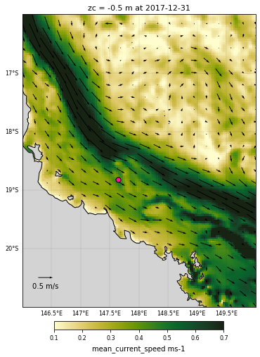
Adding a quiver plot on top

To make the quiver plot, we will first resample the dataset and take one point every 7 times. It allows to have less arrows on the map making it more readable.

# Figure size
size = (7, 8)

# Time step to plot
timevar = 0

# z-coordinate position (here the top one)
zcvar = -1

# Color from cmocean
color = cmocean.cm.speed

# Defining the figure
fig = plt.figure(figsize=size, facecolor='w', 
                 edgecolor='k')

# Axes with Cartopy projection
ax = plt.axes(projection=ccrs.PlateCarree())
# and extent
ax.set_extent([min_lon, max_lon, min_lat, max_lat], 
              ccrs.PlateCarree())

# Plotting using Matplotlib the mean current
cf = ds_hydro_clip.mean_cur.isel(time=timevar,k=zcvar).plot( 
    transform=ccrs.PlateCarree(), cmap=color,
    vmin = 0.1, vmax = 0.7,
    add_colorbar=False
)

# Resampling using the slice method
resample = ds_hydro_clip.isel(time=timevar,k=zcvar,longitude=slice(None, None, 7),
                              latitude=slice(None, None, 7))

# Defining the quiver plot
quiver = resample.plot.quiver(x='longitude', y='latitude', u='u', v='v', 
                              transform=ccrs.PlateCarree(), scale=8)      

# Vector options declaration
veclenght = 0.5
maxstr = '%3.1f m/s' % veclenght
plt.quiverkey(quiver,0.1,0.1,veclenght,maxstr,labelpos='S', 
              coordinates='axes').set_zorder(11)


# Color bar
cbar = fig.colorbar(cf, ax=ax, fraction=0.027, pad=0.045, 
                    orientation="horizontal")
cbar.set_label(ds_hydro_clip.mean_cur.long_name+' '+
               ds_hydro_clip.mean_cur.units, rotation=0, 
               labelpad=5, fontsize=10)
cbar.ax.tick_params(labelsize=8)

# Title
plt.title('zc = '+str(ds_hydro_clip.mean_cur.zc.values.item(zcvar))+' m at '+
          str(ds_hydro_clip.mean_cur.coords['time'].values[timevar])[:10],
          fontsize=11
         )

# Plot lat/lon grid 
gl = ax.gridlines(crs=ccrs.PlateCarree(), draw_labels=True,
                  linewidth=0.1, color='k', alpha=1, 
                  linestyle='--')
gl.top_labels = False
gl.right_labels = False
gl.xformatter = LONGITUDE_FORMATTER
gl.yformatter = LATITUDE_FORMATTER
gl.xlabel_style = {'size': 8}
gl.ylabel_style = {'size': 8} 

# Add map features with Cartopy 
ax.add_feature(cfeature.NaturalEarthFeature('physical', 'land', '10m', 
                                            edgecolor='face', 
                                            facecolor='lightgray'))
ax.coastlines(linewidth=1)

# Site Davies Reef
ax.scatter(reef_lon, reef_lat, c='deeppink', s=50, edgecolors='k', 
           linewidth=1, transform=ccrs.PlateCarree()).set_zorder(11)

plt.tight_layout()
plt.show()
fig.clear()
plt.close(fig)
plt.clf()

<Figure size 432x288 with 0 Axes>

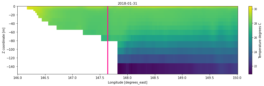
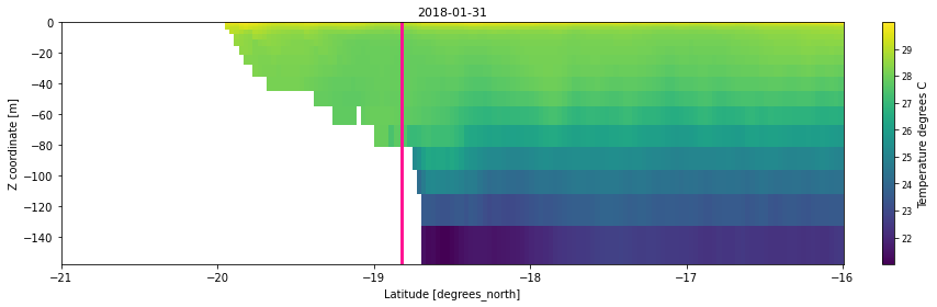
Cross-sections on Xarray dataset

To define the cross-section, we chose to select (sel) several latitudes or longitudes and compute the mean along the opposite dimension:

# Section along the longitude
lonsec = ds_bio_clip.sel(latitude=slice(*[-19.,-18.5])).mean(dim=('latitude'),skipna=True)

# Section along the latitude
latsec = ds_bio_clip.sel(longitude=slice(*[147.2,148.])).mean(dim=('longitude'),skipna=True)

Let’s visualise the selected mean cross-sections:

# Figure size
size = (12, 4)

# Time step to plot
timevar = -1

# Color from cmocean
color = cmocean.cm.speed

# Defining the figure
fig = plt.figure(figsize=size, facecolor='w', edgecolor='k')
ax = plt.axes()

# Plotting using Matplotlib the temperature over the z-coordinate
sec = lonsec.temp.isel(time=timevar).plot(y="zc", add_colorbar=False)

# Color bar
cbar = fig.colorbar(sec, ax=ax, fraction=0.027, pad=0.045)
cbar.set_label(ds_bio.temp.long_name+' '+
               ds_bio.temp.units, rotation=90, 
               labelpad=5, fontsize=10)
cbar.ax.tick_params(labelsize=8)

# Title
plt.title(str(lonsec.temp.coords['time'].values[timevar])[:10],
          fontsize=11
         )

# Site Davies Reef visualised as a line
ax.plot([reef_lon,reef_lon], [-1000,16], c='deeppink',  
           linewidth=3)

plt.tight_layout()
plt.show()
fig.clear()
plt.close(fig)
plt.clf()

<Figure size 432x288 with 0 Axes>

# Figure size
size = (12, 4)

# Time step to plot
timevar = -1

# Color from cmocean
color = cmocean.cm.speed

# Defining the figure
fig = plt.figure(figsize=size, facecolor='w', edgecolor='k')
ax = plt.axes()

# Plotting using Matplotlib the temperature over the z-coordinate
sec = latsec.temp.isel(time=timevar).plot(y="zc",add_colorbar=False)

# Color bar
cbar = fig.colorbar(sec, ax=ax, fraction=0.027, pad=0.045)
cbar.set_label(ds_bio.temp.long_name+' '+
               ds_bio.temp.units, rotation=90, 
               labelpad=5, fontsize=10)
cbar.ax.tick_params(labelsize=8)

# Title
plt.title(str(latsec.temp.coords['time'].values[timevar])[:10],
          fontsize=11
         )

# Site Davies Reef visualised as a line
ax.plot([reef_lat,reef_lat], [-1000,16], c='deeppink',  
           linewidth=3)

plt.tight_layout()
plt.show()
fig.clear()
plt.close(fig)
plt.clf()

<Figure size 432x288 with 0 Axes>

Xarray Davies Reef Interactive maps