eReefs model description
This material is from the eReefs.org.au website and the eReefs Research from CSIRO.
eReefs Hydrodynamic and BioGeoChemical models of the Great Barrier Reef are like weather models, but for the marine environment, providing a picture of the current and historical environmental conditions on the Great Barrier Reef. For example you can use these models to investigate past extreme weather events such as:
Cyclones: Yasi (Feb 2011), Ita (April 2014), Nathan (March 2015), Debbi (March 2017),
%%HTML
<div align="middle">
<video width="100%" controls>
      <source src="https://aims-ereefs-public-prod.s3.amazonaws.com/ncanimate/products/products__ncanimate__ereefs__gbr4_v2__temp-wind-salt-current_hourly/products__ncanimate__ereefs__gbr4_v2__temp-wind-salt-current_hourly_video_monthly_2011-02_queensland-1_-1.5.mp4?t=1599128595287" type="video/mp4">
</video></div>
Coral bleaching from high temperature (March 2016, March 2017),
%%HTML
<div align="middle">
<video width="100%" controls>
      <source src="https://aims-ereefs-public-prod.s3.amazonaws.com/ncanimate/products/products__ncanimate__ereefs__gbr4_v2__temp-wind-salt-current_hourly/products__ncanimate__ereefs__gbr4_v2__temp-wind-salt-current_hourly_video_monthly_2017-03_queensland-1_-1.5.mp4?t=1599549818184" type="video/mp4">
</video></div>
Flood plumes with low salinity (North Queensland Flooding 2019, Burdekin Jan 2011)
%%HTML
<div align="middle">
<video width="100%" controls>
      <source src="https://aims-ereefs-public-prod.s3.amazonaws.com/ncanimate/products/products__ncanimate__ereefs__gbr1_2-0__salt-multi-depth_hourly/products__ncanimate__ereefs__gbr1_2-0__salt-multi-depth_hourly_video_monthly_2019-02_townsville-3_0.mp4?t=1599405869920" type="video/mp4">
</video></div>
eReefs CSIRO Hydrodynamic model
The eReefs hydrodynamic model predicts the movement of water and key environmental conditions (temperature, salinity, currents, tides). This model allows us to better understand how cyclones mix the water, the location of potentially damaging heat waves, the ocean currents that disperse larvae of corals and Crown-of-Thorns starfish, and fresh water plumes from flooded rivers that can damage inshore reefs.
This model is run with a 4 km and 1 km grid size. The 4 km grid has a longer hindcast going back to September 2010, while the 1 km model starts in December 2014. The 1 km model also only extends out to the edge of the Great Barrier Reef, whereas the 4 km model covers much of the Coral Sea. The hydrodynamic model and visualisations are normally updated in near-real time, within 1 week of the current date.
Note
The eReefs models are currently not being run in near-real time by CSIRO and most of the available dataset are available up to mid 2020. Near realtime results are expected to be back in operation this year.
Regional hydrodynamics
The general circulation of the Great Barrier Reef region is summarized in Figure 1.
The South Equatorial Current flows westwards through the Coral Sea as a number of narrow current jets controlled by the complex plateaux, seamounts and ridge topography of this ocean basin, with the most significant of these jets occurring immediately north and south of the Queensland Plateau.
On approaching the western boundary of the Coral Sea, these multiple jets are steered by the Australian continental shelf to form the southward flowing East Australian Current (EAC) and the northward flowing Hiri Current. The Hiri Current flows along the shelf edge of the northern GBR into the Gulf of Papua where it forms a semi-closed cyclonic eddy.
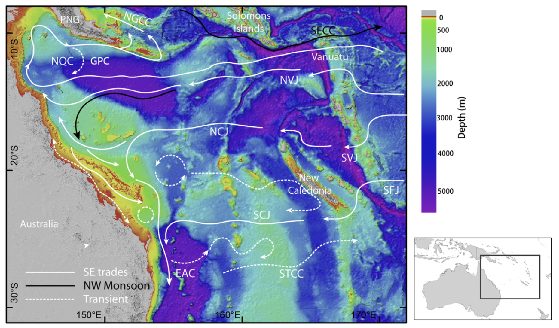
Fig. 1 Bathymetry and key currents in the Great Barrier Reef region NGCC: New Guinea Coastal Current, mirroring the deeper New Guinea Coastal Undercurrent; NQC: NorthQueensland Current which is part of the Gulf of Papua Current (GPC); SECC: South Equatorial Countercurrent; Jets of the South Equatorial Current (SEC): NVJ: North Vanuatu Jet; NCJ: North Caledonia Jet; SVJ: South Vanuatu Jet; SFJ: South Fiji Jet; SCJ: South Caledonia Jet; EAC: East Australian Current; STCC: Subtropical Counter current; A wind-driven coastal current is shown running parallel to the coast along the inner shelf (bathymetry data courtesy of 1) 2.
More information about GBR hydrodynamics
For a detailed description of the circulation in the Great Barrier Reef and its regional consequences, you need to go through the CSIRO eReefs Research page on the subject.
SHOC model
The eReefs project relies on the hydrodynamic model SHOC (Sparse Hydrodynamic Ocean Code 3) for both the regional and shelf model applications.
SHOC is a general purpose model (Herzfeld, 2006) applicable on spatial scales ranging from estuaries to regional ocean domains. It is a three-dimensional finite-difference hydrodynamic model based on the equations of momentum, continuity and conservation of heat and salt, employing the hydrostatic and Boussinesq assumptions.
Model inputs
Inputs required by the model include forcing due to:
wind,
atmospheric pressure gradients,
surface heat and water fluxes and
open-boundary conditions such as tides and low frequency ocean currents.
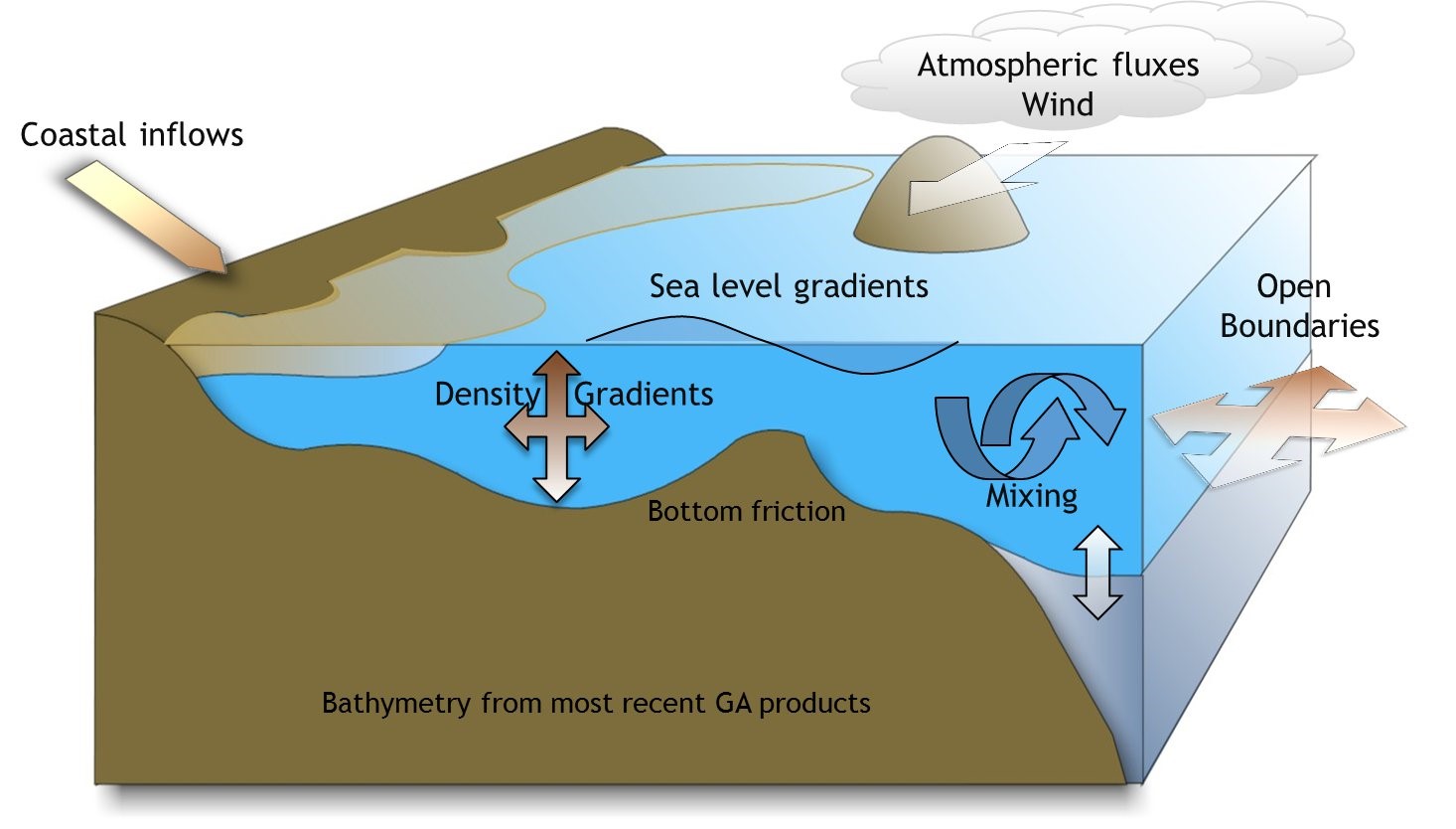
Fig. 2 Schematic representation of major forcing inputs for the SHOC hydrodynamic model.
Model inputs
Outputs from the model include three-dimensional distributions of:
velocity,
temperature,
salinity,
density,
passive tracers,
mixing coefficients and
sea-level.
eReefs regional marine models
The model uses a curvilinear orthogonal grid in the horizontal and a fixed z coordinates in the vertical (vertical grid types). The z vertical system allows for wetting and drying of surface cells, useful for modelling regions such as tidal flats where large areas are periodically dry.
Two resolutions have been chosen for the regional model (1km and 4km, see Fig. 3 below).
The GBR1 grid is extremely large, with size 510 x 2390. There are 48 vertical layers, with 1 m resolution at the surface. Although the grid is large, only 50% of the surface cells and 22% of the full 3D domain is in fact wet.
The GBR4 grid is less computationally demanding; size is 220 x 500 x 44 with 1 m vertical resolution at the surface. As mentioned above, both models employ orthogonal curvilinear grids over the domain.
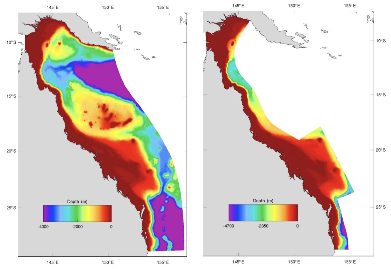
Fig. 3 Model grid and bathymetry for the 4km (left) and 1km (right) resolution model.
Hydrodynamic models of 4 km and 1 km forced by OceanMAPS global model, ACCESS meteorology and 25 rivers.
Hindcast from Sep 2010 - present day.
Near real time.
4 km version resolves interaction of large rivers, reef matrix, shelf and open ocean.
Suitable for broad scale investigations,
Computationally efficient,
Bridging model for global model.
1 km resolves individual reefs, river plumes etc.
Suitable for more regional scale investigations,
Computationally inefficient.
Model descriptions
Several slides explaining the eReefs Regional Models are available in a 2016 Workshop Presentations.
eReefs CSIRO BioGeoChemical model (4 km)
The GBR4 BioGeoChemical (GBR) model builds on the GBR4 hydrodynamic model by modelling the water quality (nutrients and suspended sediment) and key ecological processes (coral, seagrass, plankton) that drive the water chemistry. This model allows us to better understand how water quality is affected by land runoff. Detailed information about the model can be found in the paper: CSIRO Environmental Modelling Suite (EMS): Scientific description of the optical and biogeochemical models (vB3p0).
In this course, we will be using the version 3.1 of the BioGeoChemical (BGC) model. Version 3.1 of the BGC was developed to compare the effects of land practice improvements on water quality changes in the Great Barrier Reef. It was run with three scenarios of river sediment and nutrient loads to simulate the differences between:
baseline conditions (based on current land use practices in 2019),
pre-industrial catchment conditions, and
target catchment conditions (anthropogenic loads reduced according to the percentage reductions of DIN, PN, PP and TSS specified in the Reef 2050 Water Quality Improvement Plan 2017-2022).
A technical assessment of the skill level of the BGC version 3.1 model shows that the absolute accuracy of the BGC model varies significantly with variable and location. An older analysis on the BGC version 2.0 (Skerratt et al., 2018) provides additional background on the skill of the BGC model. As a result care should be taken to ensure the model is fit-for-purpose and in general BGC results should used in combination with second sources of information for making recommendations.
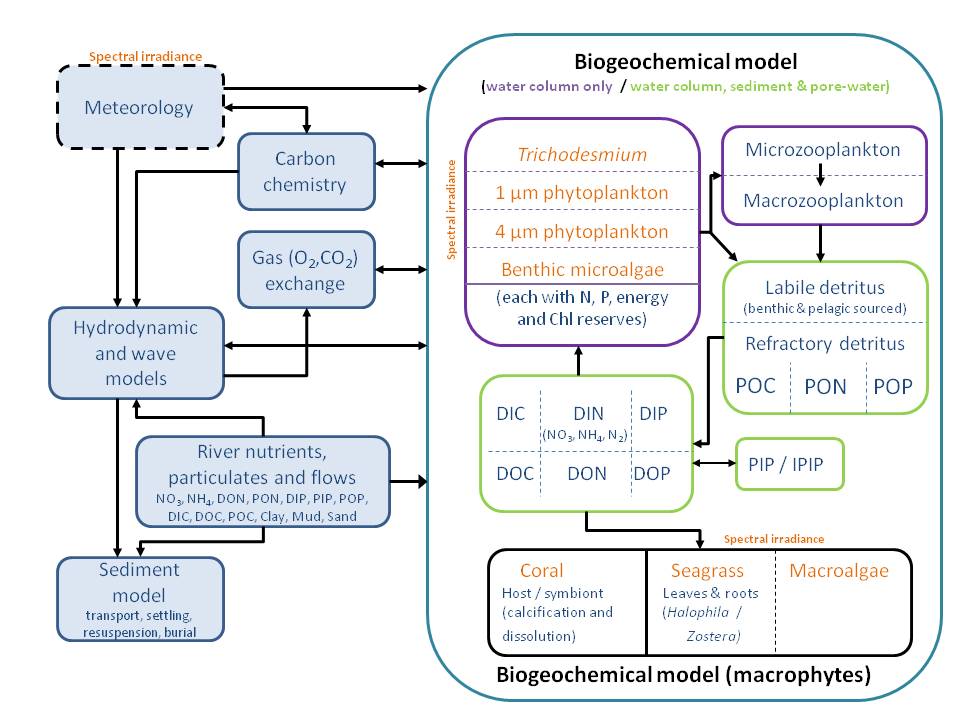
Fig. 4 Schematic diagram of the ecological model compartments, links and vertical layers.
More information about biogeochemistry and ecology
For a detailed description of the ecological processes represented in the biogeochemical model, you need to go through the CSIRO eReefs Research page on the subject.
Components integration overview
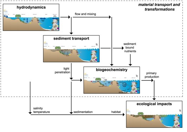
Fig. 5 Primary components of a material transport and transformation models (inside box), and showing internal linkages between sub models and linkage to ecological impacts models (from 4).
Reef management challenges for which the eReefs modelling suite has application are numerous and include prediction of coral bleaching hotspots, impacts of ocean acidification on coral calcification, catchment impacts on reef health (sedimentation issues, eutrophication), crown of thorns starfish (COTS) infestations, hypoxia, management of dredging, shipping and port related activities, fisheries management, search and rescue, larval connectivity and prediction of impacts of floods or extreme weather events on marine systems. Since the modelling package operates routinely in near real-time, emergent events such as floods, dredge plumes, phytoplankton blooms, cyclones, vessel groundings, bleaching events etc. may be investigated and responded to in a timely manner.
Important
Maintaining a current archive of the state of the Great Barrier Reef assures that any investigations of processes and dynamics remain relevant, and account for shifts in the state of the system.
- 1
Beaman, R.J., 2010: Project 3DGBR: A high-resolution depth model for the Great Barrier Reef and Coral Sea. Marine and Tropical Sciences Research Facility (MTSRF), Project 2.5i.1a, Final Report, MTSRF, Cairns, Australia, pp. 13 plus Appendix 1.
- 2
Schiller et al., 2015: Cross-shelf exchanges between the Coral Sea and the Great Barrier Reef lagoon determined from a regional-scale numerical model, Continental Shelf Research, 109, 150-163, DOI
- 3
Herzfeld, M. (2006) An alternative coordinate system for solving finite difference ocean models. Ocean Modelling, 14, 174 – 196.
- 4
Webster, I.T., Brinkman, R., Parslow, J., Prange, J., Stevens, A.D.L., Waterhouse, J. 2008. Review and Gap Analysis of Receiving-Water Water Quality Modelling in the Great Barrier Reef. CSIRO Water for a Healthy Country Flagship. 137 p.