IMOS Ocean Radar Data Query
This notebook is based on the examples from the IMOS based Python library tutorial.
Introduction
The Australian Coastal Ocean Radar Network (ACORN) facility comprises a coordinated network of HF radars delivering real-time ocean surface velocity data.
In this third example (OceanData2.ipynb), we will export the dataset file (NetCDF) for a given region and then we will plot the velocity field at a given time in a latitude/longitude grid.
The Australian Coastal Ocean Radar Network (ACORN) facility comprises a coordinated network of HF radars delivering:
real-time, non-quality controlled and
delayed-mode, quality controlled surface current data into a national archive.
NetCDF files can be found at : http://thredds.aodn.org.au/thredds/catalog/IMOS/ACORN/catalog.html
Monthly aggregated files are also available in the following folders: http://thredds.aodn.org.au/thredds/catalog/IMOS/ACORN/gridded_1h-avg-current-map_non-QC/catalog.html

Content:
Loading required modules for this exercise
%matplotlib inline

import cmocean as cmo
from netCDF4 import Dataset
from netCDF4 import num2date
import matplotlib.pyplot as plt

%matplotlib inline
%config InlineBackend.figure_format = 'svg'
plt.rcParams['mathtext.fontset'] = 'cm'
Data access is provided via HTTP and OPeNDAP by THREDDS Data Server and FTP. Key transfer protocols acronyms:
HTTP: Hypertext Transfer Protocol
OPenDAP: Open-source Project for a Network Data Access Protocol
THREDDS: Thematic Real-Time Environmental Distributed Data Services
FTP: File Transfer Protocol
LAS: Live Access Server
ACORN data from IMOS
Following previous example, we first export the NetCDF dataset from the IMOS AODN THREDDS data server.
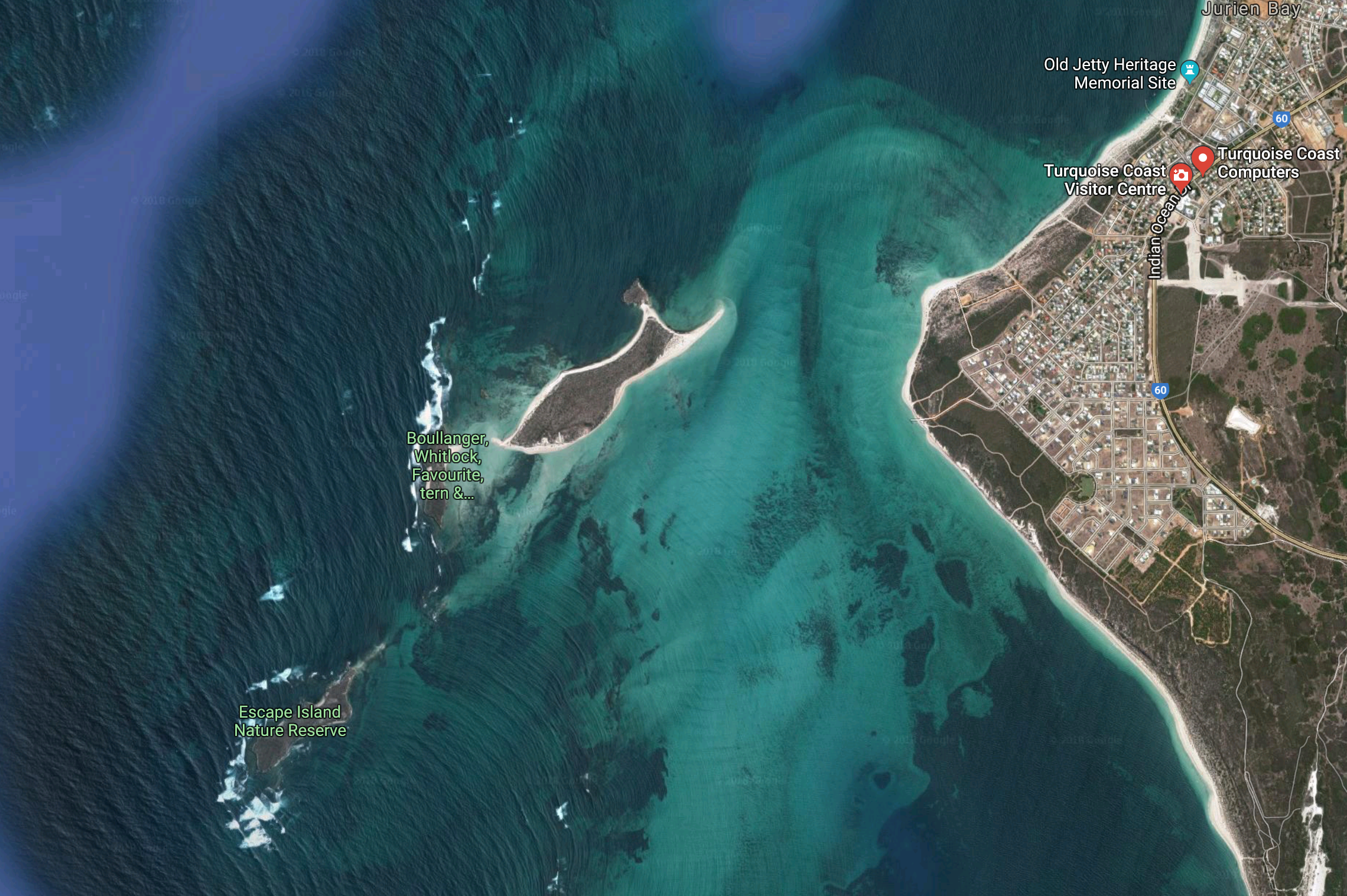
Fig. 3 Turquoise Bay
The catalog containing all the ACORN dataset is found on the link below:
http://thredds.aodn.org.au/thredds/catalog/IMOS/ACORN/gridded_1h-avg-current-map_non-QC/catalog.html
You will note that there are several folders corresponding to different radar sites. We will use the dataset from Turquoise Coast in WA.
As shown in the video below, navigate through the folder and pick a year, month and day.
from IPython.display import YouTubeVideo
YouTubeVideo('qiw0yGzfZak', width=760, height=450)
# Paste the Turquoise Coast dataset URL
acorn_URL = 'http://thredds.aodn.org.au/thredds/dodsC/IMOS/ACORN/gridded_1h-avg-current-map_non-QC/TURQ/2021/02/11/IMOS_ACORN_V_20210211T140000Z_TURQ_FV00_1-hour-avg.nc'

# Export the NetCDF file in Python
acorn_DATA = Dataset(acorn_URL+'#fillmismatch')
The first thing to notice is the distinctive Data Reference Syntax (DRS) associated with the file. Staff at IMOS have archived the data according to the following directory structure:
http://thredds.aodn.org.au/thredds/dodsC/organisation/project/collection/site-code/year/month/day/
From this we can deduce, without even inspecting the content of the file, who is the data provider, when and where it was collected.
Tip
While it’s unlikely that your research will ever involve cataloging data from such a large observational network, it’s still a very good idea to develop your own personal DRS for the data you do have.
This often involves investing some time at the beginning of a project to think carefully about the design of your directory and file name structures, as these can be very hard to change later on. Well planned DRS is one of the easiest ways to make your work more efficient and reliable.
In order to see all the global attributes and some other information about the file, type in your command window
# Discover Metadata
print(acorn_DATA)
<class 'netCDF4._netCDF4.Dataset'>
root group (NETCDF3_CLASSIC data model, file format DAP2):
    project: Integrated Marine Observing System (IMOS)
    Conventions: CF-1.6,IMOS-1.4
    institution: Australian Coastal Ocean Radar Network (ACORN)
    title: IMOS ACORN Turqoise Coast (TURQ), one hour averaged current RT-QC data, 2021-02-11T14:00:00Z
    instrument: CODAR Ocean Sensors/SeaSonde
    site_code: TURQ, Turqoise Coast
    ssr_Stations: Lancelin (LANC), Green Head (GHED)
    date_created: 2021-02-11T15:30:19Z
    abstract: The ACORN facility is producing NetCDF files containing vector current maps at 1 hour time interval for time instant 2021-02-11 14:00:00Z in the region extending between Longitude: (112.124,115.827) and Latitude:(-32.515,-29.307). The final product is produced on a regular geographic grid. They are produced from radial currents in the Turquoise Coast (WA), which represent the surface sea water current component along the radial direction from a receiver antenna. Radials are calculated from the shift of the Bragg peaks in a power spectrum. They are mapped onto specific angles through a Direction-Finding algorithm and are converted into current vector components using an unweighted least-squares fit. Radials and vector maps are computed using the standard software provided by the ocean radar manifacturer, CODAR Ocean Sensors (COS). Radials are extracted from the Doppler spectra using the calibrated antenna pattern. Thresholds for radial SNR and velocities are set to 6dB, and 150 cm s-1. Vectors are produced at each grid point using an unweighted least-squares fit. Radial velocities from the two sites falling within a search radius R=20 km around each grid point are used in the computation. At least two radials per site are required in computation of the velocity components. QC procedures apply first to intersection angle (GDOP>=30 & GDOP<=150); a threshold of 150 cm s-1 is applied on current velocity. the U, V current components are then flagged based on the number of radial velocities from each site that contribute to the velocity vector. Quality flag is set to 4 if NOBS1==1 or NOBS2==1; it is set to 3 if NOBS1/NOBS2>=10 or NOBS2/NOBS1<=10; it is set to 2 if (NOBS1/NOBS2>=1 & NOBS2/NOBS1<10), or if (NOBS2/NOBS1>=1 & NOBS1/NOBS2<10). The final product is produced on a regular geographic grid. More information on the data processing is available through the document: Quality Control procedures for ACORN radars Manual Version 1.3.3. Integrated Marine Observing System. DOI: 10.26198/5c89b59a931cb (http://dx.doi.org/10.26198/5c89b59a931cb).
    source: Terrestrial HF radar
    keywords: Oceans
    standard_name_vocabulary: NetCDF Climate and Forecast (CF) Metadata Convention Standard Name Table 27
    netcdf_version: 4.3.3.1
    naming_authority: IMOS
    file_version: Level 0 - RT Quality Controlled data
    file_version_quality_control: Data in this file has been through the quality control procedure as described in the document: Quality Control procedures for ACORN radars Manual Version 1.3.3. Integrated Marine Observing System. DOI: 10.26198/5c89b59a931cb (http://dx.doi.org/10.26198/5c89b59a931cb).  Every data point in this file has an associated quality flag.
    geospatial_lat_min: -32.5151159
    geospatial_lat_max: -29.3070009
    geospatial_lat_units: degrees_north
    geospatial_lon_min: 112.1237434
    geospatial_lon_max: 115.8266081
    geospatial_lon_units: degrees_east
    geospatial_vertical_min: 0.0
    geospatial_vertical_max: 0.0
    geospatial_vertical_units: m
    time_coverage_start: 2021-02-11T14:00:00Z
    time_coverage_end: 2021-02-11T14:00:00Z
    local_time_zone: 8.0
    data_centre_email: info@aodn.org.au
    data_centre: Australian Ocean Data Network (AODN)
    author: Cosoli, Simone
    author_email: simone.cosoli@uwa.edu.au
    institution_references: http://www.imos.org.au/acorn.html
    principal_investigator: Cosoli, Simone
    citation: The citation in a list of references is: IMOS, [year-of-data-download], [Title], [data-access-URL], accessed [date-of-access]
    acknowledgement: Any users (including re-packagers) of IMOS data are required to clearly acknowledge the source of the material in this format: "Data was sourced from the Integrated Marine Observing System (IMOS) - IMOS is supported by the Australian Government through the National Collaborative Research Infrastructure Strategy and the Super Science Initiative."
    distribution_statement: Data may be re-used, provided that related metadata explaining the data has been reviewed by the user, and the data is appropriately acknowledged. Data, products and services from IMOS are provided "as is" without any warranty as to fitness for a particular purpose.
    comment: This NetCDF file has been created using the IMOS NetCDF Conventions v1.4.
    disclaimer: Data, products and services from IMOS are provided "as is" without any warranty as to fitness for a particular purpose.
    license: http://creativecommons.org/licenses/by/4.0/
    DODS_EXTRA.Unlimited_Dimension: TIME
    dimensions(sizes): TIME(1), I(60), J(59)
    variables(dimensions): float64 TIME(TIME), int32 I(I), int32 J(J), float64 LATITUDE(I, J), float64 LONGITUDE(I, J), float32 GDOP(I, J), float32 UCUR(TIME, I, J), float32 VCUR(TIME, I, J), float32 UCUR_sd(TIME, I, J), float32 VCUR_sd(TIME, I, J), int8 NOBS1(TIME, I, J), int8 NOBS2(TIME, I, J), int8 UCUR_quality_control(TIME, I, J), int8 VCUR_quality_control(TIME, I, J)
    groups:
To list all the variables available in the NetCDF file, type:
# Discover variables
print(acorn_DATA.variables.keys())
odict_keys(['TIME', 'I', 'J', 'LATITUDE', 'LONGITUDE', 'GDOP', 'UCUR', 'VCUR', 'UCUR_sd', 'VCUR_sd', 'NOBS1', 'NOBS2', 'UCUR_quality_control', 'VCUR_quality_control'])
As we have seen already on of the great thing about netCDF files is that they contain metadata - that is, data about the data. They are global attributes that give information about the file as a whole, while each variable also has its own attributes.
As an example, we plot the attributes associated to the TIME variable:
print('These are the attributes of the time axis:')
print(acorn_DATA.variables['TIME'])

print('--------')

print('Here is the first time value:')
print(acorn_DATA.variables['TIME'][0])
These are the attributes of the time axis:
<class 'netCDF4._netCDF4.Variable'>
float64 TIME(TIME)
    standard_name: time
    long_name: time
    units: days since 1950-01-01 00:00:00 UTC
    axis: T
    valid_min: 0.0
    valid_max: 999999.0
    calendar: gregorian
    comment: Given time lays at the middle of the averaging time period.
    local_time_zone: 8.0
    _ChunkSizes: 524288
unlimited dimensions: TIME
current shape = (1,)
filling off
--------
Here is the first time value:
25974.583333333372
The raw time value are fairly meaningless, but we can use the time attributes to convert them to a more meaningful format…
units = acorn_DATA.variables['TIME'].units
calendar = acorn_DATA.variables['TIME'].calendar

times = num2date(acorn_DATA.variables['TIME'][:], units=units, calendar=calendar)

print('Meaningfull dataset time:')
print(times[0])
Meaningfull dataset time:
2021-02-11 14:00:00.000003
Get current speed
First we will need to find the zonal (east/west) and meridional (north/south) surface current components in our dataset. To do so you will have to use the acorn_DATA.variables['XXX'] function as above where XXX is one of the available variables.
print(acorn_DATA.variables['UCUR'])
<class 'netCDF4._netCDF4.Variable'>
float32 UCUR(TIME, I, J)
    _FillValue: 999999.0
    standard_name: eastward_sea_water_velocity
    long_name: Mean of sea water velocity U component values in 1 hour, after rejection of obvious bad data (see abstract).
    units: m s-1
    valid_min: -10.0
    valid_max: 10.0
    cell_methods: TIME: mean
    ancillary_variables: UCUR_quality_control
    coordinates: TIME LATITUDE LONGITUDE
    _ChunkSizes: [ 1 60 59]
unlimited dimensions: TIME
current shape = (1, 60, 59)
filling off
print(acorn_DATA.variables['VCUR'])
<class 'netCDF4._netCDF4.Variable'>
float32 VCUR(TIME, I, J)
    _FillValue: 999999.0
    standard_name: northward_sea_water_velocity
    long_name: Mean of sea water velocity V component values in 1 hour, after rejection of obvious bad data (see abstract).
    units: m s-1
    valid_min: -10.0
    valid_max: 10.0
    cell_methods: TIME: mean
    ancillary_variables: VCUR_quality_control
    coordinates: TIME LATITUDE LONGITUDE
    _ChunkSizes: [ 1 60 59]
unlimited dimensions: TIME
current shape = (1, 60, 59)
filling off
Let us define Numpy variables for each of these NetCDF variables.
uData = acorn_DATA.variables['UCUR'][:,:,:]
vData = acorn_DATA.variables['VCUR'][:,:,:]
uData.shape
(1, 60, 59)
Both uData and vData are a special type of Numpy array known as a masked array, whereby some of the points in the latitude/longitude grid have missing (or masked) values.
Just as with a normal Numpy array, we can check the shape of our data (in fact, masked arrays can do everything normal Numpy arrays can do and more).
print(type(uData))
print(uData.shape)
<class 'numpy.ma.core.MaskedArray'>
(1, 60, 59)
In other words, the dataset contains 1 time step, 60 latitudes and 59 longitudes.
We can now go ahead and calculate the current speed \(s\): $\( s = \sqrt{u^2+v^2} \)$
sData = (uData**2 + vData**2)**0.5
Plotting Turquoise Coast dataset
Tip
It’s a good idea to regularly view your data throughout the code development process, just to ensure nothing crazy has happened along the way.
# Get the grid values (long/lat)
LAT = acorn_DATA.variables['LATITUDE']
LON = acorn_DATA.variables['LONGITUDE']
TIME = acorn_DATA.variables['TIME']
latData = LAT[:]
lonData = LON[:]

# Grab the units for current velocity
units = acorn_DATA.variables['UCUR'].units

figure = plt.figure(figsize=(8, 8), facecolor='w', edgecolor='k')

# Plot the calculated current speed
plt.pcolor(lonData , latData, sData[0,:,:], cmap=cmo.cm.matter, shading='nearest')
plt.tick_params(axis='both', which='major', labelsize=8)
cbar = plt.colorbar()
cbar.ax.set_ylabel('Current speed in ' + units, fontsize=8)
cbar.ax.tick_params(labelsize=7)

# Use metadata information as well as time to write the figure title
plt.title(acorn_DATA.title + '\n' + num2date(TIME[0], TIME.units, TIME.calendar).strftime('%d/%m/%Y'), fontsize=10)
plt.xlabel(LON.long_name + ' in ' + LON.units, fontsize=8)
plt.ylabel(LAT.long_name + ' in ' + LAT.units, fontsize=8)

# Plot velocity field as arrows based on zonal and meridional velocity components
Q = plt.quiver(lonData, latData, uData[0,:,:], vData[0,:,:], units='width')

plt.show()
plt.close()
/usr/share/miniconda/envs/coast/lib/python3.6/site-packages/ipykernel_launcher.py:14: UserWarning: The input coordinates to pcolor are interpreted as cell centers, but are not monotonically increasing or decreasing. This may lead to incorrectly calculated cell edges, in which case, please supply explicit cell edges to pcolor.

Note
You can now try to plot 1h averaged sea water speed gridded data from ACORN data at another time interval or on another location and do some data crunching with it!